Puedes personalizar la apariencia de tus gráficos hechos con ggplot2 usando temas creados por los usuarios. Haz click sobre los botones de cada sección para previsualizar el tema y su código correspondiente.
Ten en cuenta que puedes sobrescribir los elementos del tema haciendo uso de la función theme, como el color de fondo, el grid o los márgenes, entre otros.
Temas predeterminados
El paquete ggplot2 proporciona ocho temas diferentes. Por defecto usa el tema llamado theme_grey (theme_gray), por lo que no necesitas especificarlo.
Elige un tema
Ten en cuenta que existe un tema adicional para usuarios avanzados llamado theme_test para realizar pruebas unitarias visuales.
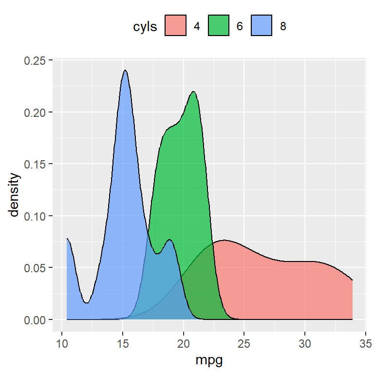
library(ggplot2)

cyls <- as.factor(mtcars$cyl)

ggplot(mtcars, aes(x = mpg, fill = cyls)) +
  geom_density(alpha = 0.7) +
  theme_grey() +  # Default
  theme(legend.position = "top")
library(ggplot2)
cyls <- as.factor(mtcars$cyl)
ggplot(mtcars, aes(x = mpg, fill = cyls)) +
geom_density(alpha = 0.7) +
theme_bw() +
theme(legend.position = "top")library(ggplot2)
cyls <- as.factor(mtcars$cyl)
ggplot(mtcars, aes(x = mpg, fill = cyls)) +
geom_density(alpha = 0.7) +
theme_linedraw() +
theme(legend.position = "top")library(ggplot2)
cyls <- as.factor(mtcars$cyl)
ggplot(mtcars, aes(x = mpg, fill = cyls)) +
geom_density(alpha = 0.7) +
theme_light() +
theme(legend.position = "top")library(ggplot2)
cyls <- as.factor(mtcars$cyl)
ggplot(mtcars, aes(x = mpg, fill = cyls)) +
geom_density(alpha = 0.7) +
theme_dark() +
theme(legend.position = "top")library(ggplot2)
cyls <- as.factor(mtcars$cyl)
ggplot(mtcars, aes(x = mpg, fill = cyls)) +
geom_density(alpha = 0.7) +
theme_minimal() +
theme(legend.position = "top")library(ggplot2)
cyls <- as.factor(mtcars$cyl)
ggplot(mtcars, aes(x = mpg, fill = cyls)) +
geom_density(alpha = 0.7) +
theme_classic() +
theme(legend.position = "top")library(ggplot2)
cyls <- as.factor(mtcars$cyl)
ggplot(mtcars, aes(x = mpg, fill = cyls)) +
geom_density(alpha = 0.7) +
theme_void() +
theme(legend.position = "top")
Paquete ggthemes
library(ggplot2)
library(ggthemes)
cyls <- as.factor(mtcars$cyl)
ggplot(mtcars, aes(x = mpg, fill = cyls)) +
geom_density(alpha = 0.7) +
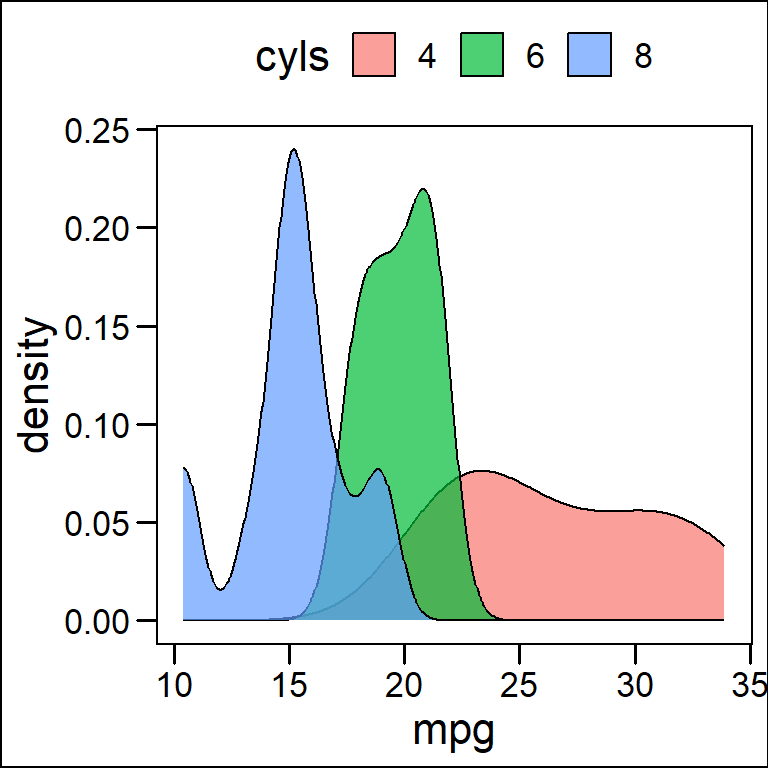
theme_base() +
theme(legend.position = "top")library(ggplot2)
library(ggthemes)
cyls <- as.factor(mtcars$cyl)
ggplot(mtcars, aes(x = mpg, fill = cyls)) +
geom_density(alpha = 0.7) +
theme_calc() +
scale_fill_calc() +
theme(legend.position = "top")library(ggplot2)
library(ggthemes)
cyls <- as.factor(mtcars$cyl)
ggplot(mtcars, aes(x = mpg, fill = cyls)) +
geom_density(alpha = 0.7) +
theme_clean() +
theme(legend.position = "top")library(ggplot2)
library(ggthemes)
cyls <- as.factor(mtcars$cyl)
ggplot(mtcars, aes(x = mpg, fill = cyls)) +
geom_density(alpha = 0.7) +
theme_economist() +
scale_fill_economist() +
theme(legend.position = "top")library(ggplot2)
library(ggthemes)
cyls <- as.factor(mtcars$cyl)
ggplot(mtcars, aes(x = mpg, fill = cyls)) +
geom_density(alpha = 0.7) +
theme_excel() +
scale_fill_excel() +
theme(legend.position = "top")library(ggplot2)
library(ggthemes)
cyls <- as.factor(mtcars$cyl)
ggplot(mtcars, aes(x = mpg, fill = cyls)) +
geom_density(alpha = 0.7) +
theme_excel_new() +
scale_fill_excel_new() +
theme(legend.position = "top")library(ggplot2)
library(ggthemes)
cyls <- as.factor(mtcars$cyl)
ggplot(mtcars, aes(x = mpg, fill = cyls)) +
geom_density(alpha = 0.7) +
theme_few() +
scale_fill_few() +
theme(legend.position = "top")library(ggplot2)
library(ggthemes)
cyls <- as.factor(mtcars$cyl)
ggplot(mtcars, aes(x = mpg, fill = cyls)) +
geom_density(alpha = 0.7) +
theme_fivethirtyeight() +
scale_fill_fivethirtyeight() +
theme(legend.position = "top")library(ggplot2)
library(ggthemes)
cyls <- as.factor(mtcars$cyl)
ggplot(mtcars, aes(x = mpg, fill = cyls)) +
geom_density(alpha = 0.7) +
theme_foundation() +
theme(legend.position = "top")library(ggplot2)
library(ggthemes)
cyls <- as.factor(mtcars$cyl)
ggplot(mtcars, aes(x = mpg, fill = cyls)) +
geom_density(alpha = 0.7) +
theme_gdocs() +
scale_fill_gdocs() +
theme(legend.position = "top")library(ggplot2)
library(ggthemes)
cyls <- as.factor(mtcars$cyl)
ggplot(mtcars, aes(x = mpg, fill = cyls)) +
geom_density(alpha = 0.7) +
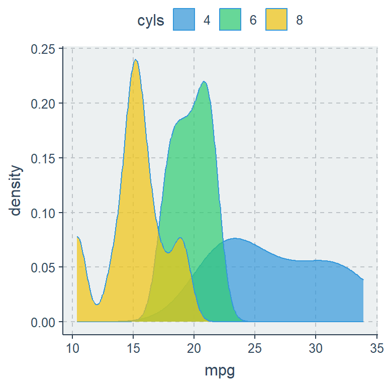
theme_hc() +
scale_fill_hc() +
theme(legend.position = "top")library(ggplot2)
library(ggthemes)
cyls <- as.factor(mtcars$cyl)
ggplot(mtcars, aes(x = mpg, fill = cyls)) +
geom_density(alpha = 0.7) +
theme_igray() +
theme(legend.position = "top")library(maps)
library(ggplot2)
library(ggthemes)
us <- fortify(map_data("state"), region = "region")
ggplot(us, aes(x = long, y = lat)) +
geom_map(map = us,
aes(fill = region,
map_id = region, group = group),
color = "black", size = 0.1) +
guides(fill = FALSE) +
theme_map() # Theme for mapslibrary(ggplot2)
library(ggthemes)
cyls <- as.factor(mtcars$cyl)
ggplot(mtcars, aes(x = mpg, fill = cyls)) +
geom_density(alpha = 0.7) +
theme_pander() +
scale_fill_pander() +
theme(legend.position = "top")library(ggplot2)
library(ggthemes)
cyls <- as.factor(mtcars$cyl)
ggplot(mtcars, aes(x = mpg, fill = cyls)) +
geom_density(alpha = 0.7) +
theme_par() +
theme(legend.position = "top")library(ggplot2)
library(ggthemes)
cyls <- as.factor(mtcars$cyl)
ggplot(mtcars, aes(x = mpg, fill = cyls)) +
geom_density(alpha = 0.7) +
theme_solarized() +
scale_fill_solarized() +
theme(legend.position = "top")library(ggplot2)
library(ggthemes)
cyls <- as.factor(mtcars$cyl)
ggplot(mtcars, aes(x = mpg, fill = cyls)) +
geom_density(alpha = 0.7) +
theme_solid() +
theme(legend.position = "top")library(ggplot2)
library(ggthemes)
cyls <- as.factor(mtcars$cyl)
ggplot(mtcars, aes(x = mpg, fill = cyls)) +
geom_density(alpha = 0.7) +
theme_stata() +
scale_fill_stata() +
theme(legend.position = "top")El paquete ggthemes contiene varios temas populares. Algunos de ellos también vienen con sus escalas de color correspondientes. Usa las escalas adecuadamente en base a tus datos.
Paquete hrbrthemes
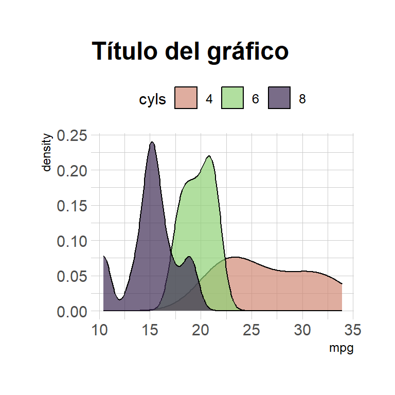
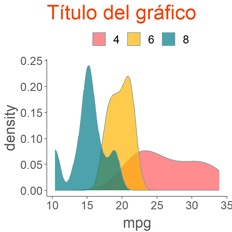
hrbrthemes proporciona “temas centrados en la tipografía y componentes de temas para ggplot2”. Los temas disponibles se muestran a continuación, pero también puedes revisar las escalas, paletas, fuentes y utilidades disponibles.
library(ggplot2)
library(hrbrthemes)

cyls <- as.factor(mtcars$cyl)

ggplot(mtcars, aes(x = mpg, fill = cyls)) +
  geom_density(alpha = 0.7) +
  ggtitle("Título del gráfico") +
  theme_ipsum() + # Arial Narrow
  scale_fill_ipsum() +
  theme(legend.position = "top")
library(ggplot2)
library(hrbrthemes)
cyls <- as.factor(mtcars$cyl)
ggplot(mtcars, aes(x = mpg, fill = cyls)) +
geom_density(alpha = 0.7) +
ggtitle("Título del gráfico") +
theme_ipsum_es() + # Econ Sans Condensed
theme(legend.position = "top")library(ggplot2)
library(hrbrthemes)
cyls <- as.factor(mtcars$cyl)
ggplot(mtcars, aes(x = mpg, fill = cyls)) +
geom_density(alpha = 0.7) +
ggtitle("Título del gráfico") +
theme_ipsum_rc() + # Roboto Condensed
theme(legend.position = "top")library(ggplot2)
library(hrbrthemes)
cyls <- as.factor(mtcars$cyl)
ggplot(mtcars, aes(x = mpg, fill = cyls)) +
geom_density(alpha = 0.7) +
ggtitle("Título del gráfico") +
theme_ipsum_ps() + # Fuente IBM Plex Sans
theme(legend.position = "top")library(ggplot2)
library(hrbrthemes)
cyls <- as.factor(mtcars$cyl)
ggplot(mtcars, aes(x = mpg, fill = cyls)) +
geom_density(alpha = 0.7) +
ggtitle("Título del gráfico") +
theme_ipsum_pub() + # Public Sans
theme(legend.position = "top")library(ggplot2)
library(hrbrthemes)
cyls <- as.factor(mtcars$cyl)
ggplot(mtcars, aes(x = mpg, fill = cyls)) +
geom_density(alpha = 0.7) +
ggtitle("Título del gráfico") +
theme_ipsum_tw() + # Titilium Web
theme(legend.position = "top")library(ggplot2)
library(hrbrthemes)
# import_roboto_condensed()
# extrafont::loadfonts(device="win")
cyls <- as.factor(mtcars$cyl)
ggplot(mtcars, aes(x = mpg, fill = cyls)) +
geom_density(alpha = 0.7) +
ggtitle("Título del gráfico") +
theme_modern_rc() + # Tema roboto Condensed dark
theme(legend.position = "top")library(ggplot2)
library(hrbrthemes)
# import_roboto_condensed()
# extrafont::loadfonts(device="win")
cyls <- as.factor(mtcars$cyl)
ggplot(mtcars, aes(x = mpg, fill = cyls)) +
geom_density(alpha = 0.7) +
ggtitle("Título del gráfico") +
theme_ft_rc() + # Tema oscuro basado en el tema FT
scale_fill_ft() +
theme(legend.position = "top")
Paquete ggthemr
library(ggplot2)
library(ggthemr)

cyls <- as.factor(mtcars$cyl)

ggthemr("flat")

ggplot(mtcars, aes(x = mpg, fill = cyls)) +
  geom_density(alpha = 0.7) +
  theme(legend.position = "top")
library(ggplot2)
library(ggthemr)
cyls <- as.factor(mtcars$cyl)
ggthemr("flat dark")
ggplot(mtcars, aes(x = mpg, fill = cyls)) +
geom_density(alpha = 0.7) +
theme(legend.position = "top")library(ggplot2)
library(ggthemr)
cyls <- as.factor(mtcars$cyl)
ggthemr("camouflage")
ggplot(mtcars, aes(x = mpg, fill = cyls)) +
geom_density(alpha = 0.7) +
theme(legend.position = "top")library(ggplot2)
library(ggthemr)
cyls <- as.factor(mtcars$cyl)
ggthemr("carrot")
ggplot(mtcars, aes(x = mpg, fill = cyls)) +
geom_density(alpha = 0.7) +
theme(legend.position = "top")library(ggplot2)
library(ggthemr)
cyls <- as.factor(mtcars$cyl)
ggthemr("chalk")
ggplot(mtcars, aes(x = mpg, fill = cyls)) +
geom_density(alpha = 0.7) +
theme(legend.position = "top")library(ggplot2)
library(ggthemr)
cyls <- as.factor(mtcars$cyl)
ggthemr("copper")
ggplot(mtcars, aes(x = mpg, fill = cyls)) +
geom_density(alpha = 0.7) +
theme(legend.position = "top")library(ggplot2)
library(ggthemr)
cyls <- as.factor(mtcars$cyl)
ggthemr("dust")
ggplot(mtcars, aes(x = mpg, fill = cyls)) +
geom_density(alpha = 0.7) +
theme(legend.position = "top")library(ggplot2)
library(ggthemr)
cyls <- as.factor(mtcars$cyl)
ggthemr("earth")
ggplot(mtcars, aes(x = mpg, fill = cyls)) +
geom_density(alpha = 0.7) +
theme(legend.position = "top")library(ggplot2)
library(ggthemr)
cyls <- as.factor(mtcars$cyl)
ggthemr("freshe")
ggplot(mtcars, aes(x = mpg, fill = cyls)) +
geom_density(alpha = 0.7) +
theme(legend.position = "top")library(ggplot2)
library(ggthemr)
cyls <- as.factor(mtcars$cyl)
ggthemr("grape")
ggplot(mtcars, aes(x = mpg, fill = cyls)) +
geom_density(alpha = 0.7) +
theme(legend.position = "top")library(ggplot2)
library(ggthemr)
cyls <- as.factor(mtcars$cyl)
ggthemr("grass")
ggplot(mtcars, aes(x = mpg, fill = cyls)) +
geom_density(alpha = 0.7) +
theme(legend.position = "top")library(ggplot2)
library(ggthemr)
cyls <- as.factor(mtcars$cyl)
ggthemr("greyscale")
ggplot(mtcars, aes(x = mpg, fill = cyls)) +
geom_density(alpha = 0.7) +
theme(legend.position = "top")library(ggplot2)
library(ggthemr)
cyls <- as.factor(mtcars$cyl)
ggthemr("light")
ggplot(mtcars, aes(x = mpg, fill = cyls)) +
geom_density(alpha = 0.7) +
theme(legend.position = "top")library(ggplot2)
library(ggthemr)
cyls <- as.factor(mtcars$cyl)
ggthemr("lilac")
ggplot(mtcars, aes(x = mpg, fill = cyls)) +
geom_density(alpha = 0.7) +
theme(legend.position = "top")library(ggplot2)
library(ggthemr)
cyls <- as.factor(mtcars$cyl)
ggthemr("pale")
ggplot(mtcars, aes(x = mpg, fill = cyls)) +
geom_density(alpha = 0.7) +
theme(legend.position = "top")library(ggplot2)
library(ggthemr)
cyls <- as.factor(mtcars$cyl)
ggthemr("sea")
ggplot(mtcars, aes(x = mpg, fill = cyls)) +
geom_density(alpha = 0.7) +
theme(legend.position = "top")library(ggplot2)
library(ggthemr)
cyls <- as.factor(mtcars$cyl)
ggthemr("sky")
ggplot(mtcars, aes(x = mpg, fill = cyls)) +
geom_density(alpha = 0.7) +
theme(legend.position = "top")library(ggplot2)
library(ggthemr)
cyls <- as.factor(mtcars$cyl)
ggthemr("solarized")
ggplot(mtcars, aes(x = mpg, fill = cyls)) +
geom_density(alpha = 0.7) +
theme(legend.position = "top")El paquete ggthemr (disponible solo en GitHub) funciona de manera diferente a otras librerías. En lugar de usar la función theme y establecer el tema puedes establecer un tema globalmente usando la función ggthemr y pasando el tema como cadena como argumento.
Ten en cuenta que tendrás que ejecutar ggthemr_reset() para volver al tema por defecto de ggplot2.
Paquete ggtech
El paquete ggtech (disponible en GitHub) proporciona temas inspirados por compañías tecnológicas, como Airbnb, Google, Twitter o Facebook.
library(ggplot2)
library(ggtech)

cyls <- as.factor(mtcars$cyl)

ggplot(mtcars, aes(x = mpg, fill = cyls)) +
  geom_density(alpha = 0.7) +
  ggtitle("Título del gráfico") +
  theme_tech(theme = "airbnb") +
  scale_fill_tech(theme = "airbnb") +
  theme(legend.position = "top")
library(ggplot2)
library(ggtech)
cyls <- as.factor(mtcars$cyl)
ggplot(mtcars, aes(x = mpg, fill = cyls)) +
geom_density(alpha = 0.7) +
ggtitle("Título del gráfico") +
theme_tech(theme = "etsy") +
scale_fill_tech(theme = "etsy") +
theme(legend.position = "top")library(ggplot2)
library(ggtech)
cyls <- as.factor(mtcars$cyl)
ggplot(mtcars, aes(x = mpg, fill = cyls)) +
geom_density(alpha = 0.7) +
ggtitle("Título del gráfico") +
theme_tech(theme = "facebook") +
scale_fill_tech(theme = "facebook") +
theme(legend.position = "top")library(ggplot2)
library(ggtech)
cyls <- as.factor(mtcars$cyl)
ggplot(mtcars, aes(x = mpg, fill = cyls)) +
geom_density(alpha = 0.7) +
ggtitle("Título del gráfico") +
theme_tech(theme = "google") +
scale_fill_tech(theme = "google") +
theme(legend.position = "top")library(ggplot2)
library(ggtech)
cyls <- as.factor(mtcars$cyl)
ggplot(mtcars, aes(x = mpg, fill = cyls)) +
geom_density(alpha = 0.7) +
ggtitle("Título del gráfico") +
theme_tech(theme = "twitter") +
scale_fill_tech(theme = "twitter") +
theme(legend.position = "top")library(ggplot2)
library(ggtech)
cyls <- as.factor(mtcars$cyl)
ggplot(mtcars, aes(x = mpg, fill = cyls)) +
geom_density(alpha = 0.7) +
ggtitle("Título del gráfico") +
theme_airbnb_fancy() +
scale_fill_tech(theme = "airbnb") +
theme(legend.position = "top")
Paquete ggdark
library(ggplot2)
library(ggdark)

cyls <- as.factor(mtcars$cyl)

ggplot(mtcars, aes(x = mpg, fill = cyls)) +
  geom_density(alpha = 0.7) +
  dark_theme_gray() +  # Default
  theme(legend.position = "top")
library(ggplot2)
library(ggdark)
cyls <- as.factor(mtcars$cyl)
ggplot(mtcars, aes(x = mpg, fill = cyls)) +
geom_density(alpha = 0.7) +
dark_theme_bw() +
theme(legend.position = "top")library(ggplot2)
library(ggdark)
cyls <- as.factor(mtcars$cyl)
ggplot(mtcars, aes(x = mpg, fill = cyls)) +
geom_density(alpha = 0.7) +
dark_theme_linedraw() +
theme(legend.position = "top")library(ggplot2)
library(ggdark)
cyls <- as.factor(mtcars$cyl)
ggplot(mtcars, aes(x = mpg, fill = cyls)) +
geom_density(alpha = 0.7) +
dark_theme_light() +
theme(legend.position = "top")library(ggplot2)
library(ggdark)
cyls <- as.factor(mtcars$cyl)
ggplot(mtcars, aes(x = mpg, fill = cyls)) +
geom_density(alpha = 0.7) +
dark_theme_dark() +
theme(legend.position = "top")library(ggplot2)
library(ggdark)
cyls <- as.factor(mtcars$cyl)
ggplot(mtcars, aes(x = mpg, fill = cyls)) +
geom_density(alpha = 0.7) +
dark_theme_minimal() +
theme(legend.position = "top")library(ggplot2)
library(ggdark)
cyls <- as.factor(mtcars$cyl)
ggplot(mtcars, aes(x = mpg, fill = cyls)) +
geom_density(alpha = 0.7) +
dark_theme_classic() +
theme(legend.position = "top")library(ggplot2)
library(ggdark)
cyls <- as.factor(mtcars$cyl)
ggplot(mtcars, aes(x = mpg, fill = cyls)) +
geom_density(alpha = 0.7) +
dark_theme_void() +
theme(legend.position = "top")library(ggplot2)
library(ggdark)
library(ggthemes)
cyls <- as.factor(mtcars$cyl)
invert_geom_defaults()
ggplot(mtcars, aes(x = mpg, fill = cyls)) +
geom_density(alpha = 0.7) +
dark_mode(theme_solarized()) +
scale_fill_solarized() +
theme(legend.position = "top")
invert_geom_defaults()ggdark proporciona el modo escuro de los temas predeterminados de ggplot2. Además, la librería puede convertir cualquier tema en un tema oscuro haciendo uso de la función dark_mode.
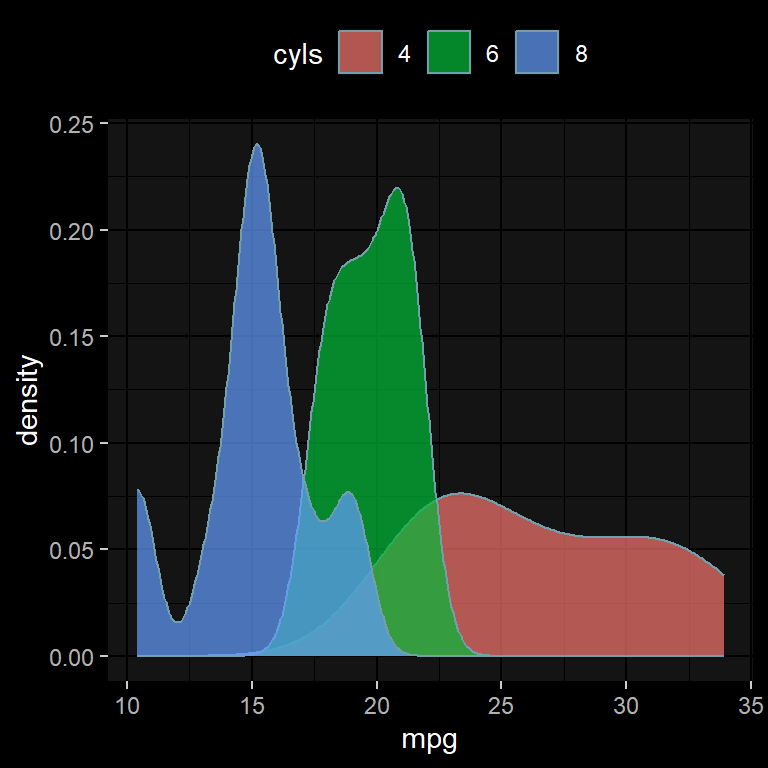
Establecer un tema activo
La función theme_set se puede usar para establecer un tema de manera global. En el siguiente ejemplo estamos estableciendo el tema predefinido theme_dark para todos los gráficos que se generen. Luego, puedes volver al tema por defecto tal y como se muestra.
library(ggplot2)

# Tema global
old <- theme_set(theme_dark())

cyls <- as.factor(mtcars$cyl)

ggplot(mtcars, aes(x = mpg, fill = cyls)) +
  geom_density(alpha = 0.7) +
  theme(legend.position = "top")

# Restablecer el tema por defecto
theme_set(old)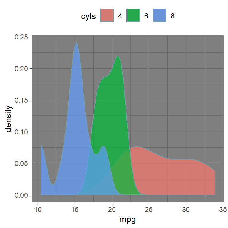

Master Statistics
Aprende estadística desde lo básico hasta técnicas avanzadas, explicado con claridad
Ir al sitio