You can customize the appearance of your plots made with ggplot2 using themes created by other users. Click on the buttons of each section to visualize each theme and its corresponding code.
Note that you can override theme elements making use of the theme function, like the background color, the grid lines or the margins, among others.
In-built themes
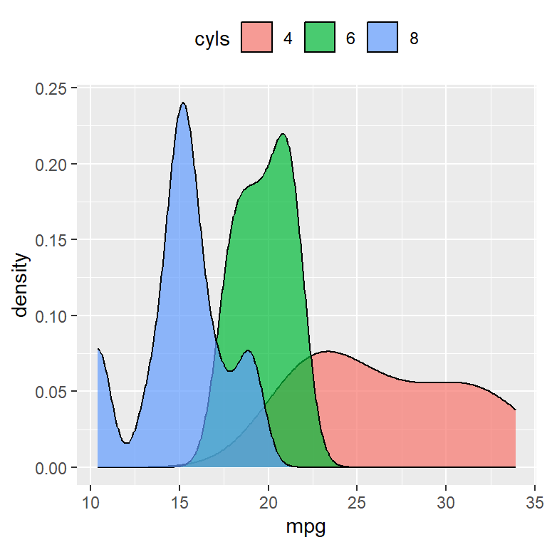
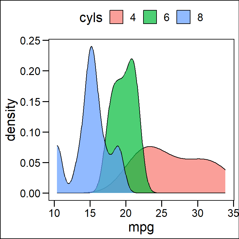
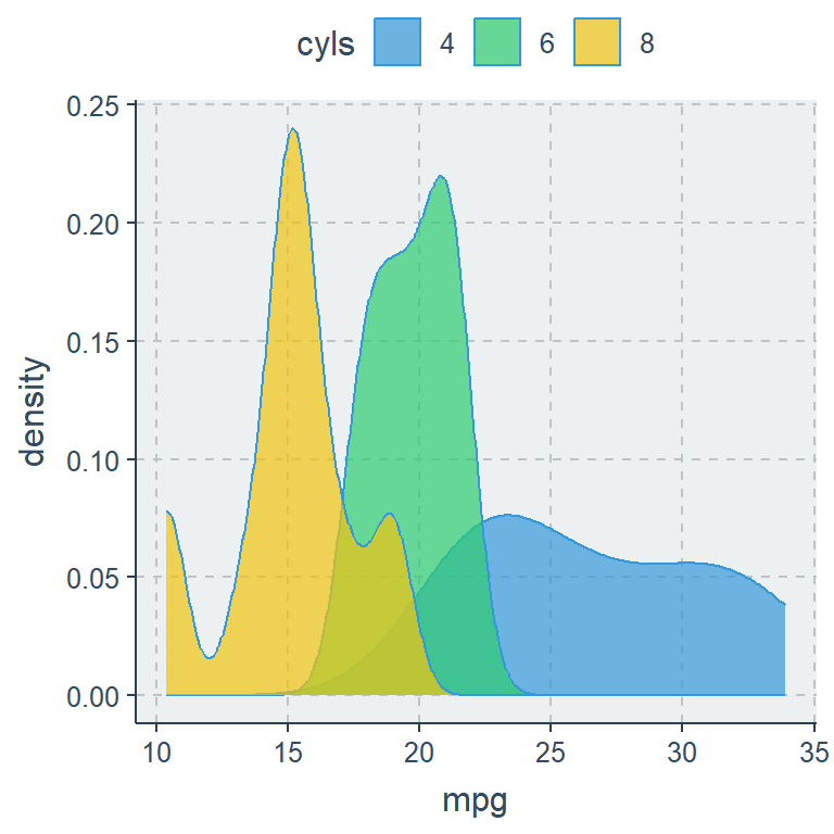
The ggplot2 package comes with eight different themes. By default it uses the theme named theme_grey (theme_gray), so you don’t really need to specify it.
Choose a theme
Note that there is an additional theme named theme_test to conduct visual unit tests by advanced users.
library(ggplot2)

cyls <- as.factor(mtcars$cyl)

ggplot(mtcars, aes(x = mpg, fill = cyls)) +
  geom_density(alpha = 0.7) +
  theme_grey() +  # Default
  theme(legend.position = "top")
library(ggplot2)
cyls <- as.factor(mtcars$cyl)
ggplot(mtcars, aes(x = mpg, fill = cyls)) +
geom_density(alpha = 0.7) +
theme_bw() +
theme(legend.position = "top")library(ggplot2)
cyls <- as.factor(mtcars$cyl)
ggplot(mtcars, aes(x = mpg, fill = cyls)) +
geom_density(alpha = 0.7) +
theme_linedraw() +
theme(legend.position = "top")library(ggplot2)
cyls <- as.factor(mtcars$cyl)
ggplot(mtcars, aes(x = mpg, fill = cyls)) +
geom_density(alpha = 0.7) +
theme_light() +
theme(legend.position = "top")library(ggplot2)
cyls <- as.factor(mtcars$cyl)
ggplot(mtcars, aes(x = mpg, fill = cyls)) +
geom_density(alpha = 0.7) +
theme_dark() +
theme(legend.position = "top")library(ggplot2)
cyls <- as.factor(mtcars$cyl)
ggplot(mtcars, aes(x = mpg, fill = cyls)) +
geom_density(alpha = 0.7) +
theme_minimal() +
theme(legend.position = "top")library(ggplot2)
cyls <- as.factor(mtcars$cyl)
ggplot(mtcars, aes(x = mpg, fill = cyls)) +
geom_density(alpha = 0.7) +
theme_classic() +
theme(legend.position = "top")library(ggplot2)
cyls <- as.factor(mtcars$cyl)
ggplot(mtcars, aes(x = mpg, fill = cyls)) +
geom_density(alpha = 0.7) +
theme_void() +
theme(legend.position = "top")
ggthemes package
library(ggplot2)
library(ggthemes)

cyls <- as.factor(mtcars$cyl)

ggplot(mtcars, aes(x = mpg, fill = cyls)) +
  geom_density(alpha = 0.7) +
  theme_base() +
  theme(legend.position = "top")
library(ggplot2)
library(ggthemes)
cyls <- as.factor(mtcars$cyl)
ggplot(mtcars, aes(x = mpg, fill = cyls)) +
geom_density(alpha = 0.7) +
theme_calc() +
scale_fill_calc() +
theme(legend.position = "top")library(ggplot2)
library(ggthemes)
cyls <- as.factor(mtcars$cyl)
ggplot(mtcars, aes(x = mpg, fill = cyls)) +
geom_density(alpha = 0.7) +
theme_clean() +
theme(legend.position = "top")library(ggplot2)
library(ggthemes)
cyls <- as.factor(mtcars$cyl)
ggplot(mtcars, aes(x = mpg, fill = cyls)) +
geom_density(alpha = 0.7) +
theme_economist() +
scale_fill_economist() +
theme(legend.position = "top")library(ggplot2)
library(ggthemes)
cyls <- as.factor(mtcars$cyl)
ggplot(mtcars, aes(x = mpg, fill = cyls)) +
geom_density(alpha = 0.7) +
theme_excel() +
scale_fill_excel() +
theme(legend.position = "top")library(ggplot2)
library(ggthemes)
cyls <- as.factor(mtcars$cyl)
ggplot(mtcars, aes(x = mpg, fill = cyls)) +
geom_density(alpha = 0.7) +
theme_excel_new() +
scale_fill_excel_new() +
theme(legend.position = "top")library(ggplot2)
library(ggthemes)
cyls <- as.factor(mtcars$cyl)
ggplot(mtcars, aes(x = mpg, fill = cyls)) +
geom_density(alpha = 0.7) +
theme_few() +
scale_fill_few() +
theme(legend.position = "top")library(ggplot2)
library(ggthemes)
cyls <- as.factor(mtcars$cyl)
ggplot(mtcars, aes(x = mpg, fill = cyls)) +
geom_density(alpha = 0.7) +
theme_fivethirtyeight() +
scale_fill_fivethirtyeight() +
theme(legend.position = "top")library(ggplot2)
library(ggthemes)
cyls <- as.factor(mtcars$cyl)
ggplot(mtcars, aes(x = mpg, fill = cyls)) +
geom_density(alpha = 0.7) +
theme_foundation() +
theme(legend.position = "top")library(ggplot2)
library(ggthemes)
cyls <- as.factor(mtcars$cyl)
ggplot(mtcars, aes(x = mpg, fill = cyls)) +
geom_density(alpha = 0.7) +
theme_gdocs() +
scale_fill_gdocs() +
theme(legend.position = "top")library(ggplot2)
library(ggthemes)
cyls <- as.factor(mtcars$cyl)
ggplot(mtcars, aes(x = mpg, fill = cyls)) +
geom_density(alpha = 0.7) +
theme_hc() +
scale_fill_hc() +
theme(legend.position = "top")library(ggplot2)
library(ggthemes)
cyls <- as.factor(mtcars$cyl)
ggplot(mtcars, aes(x = mpg, fill = cyls)) +
geom_density(alpha = 0.7) +
theme_igray() +
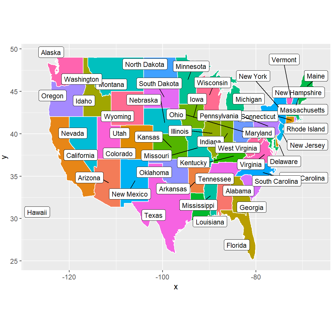
theme(legend.position = "top")library(maps)
library(ggplot2)
library(ggthemes)
us <- fortify(map_data("state"), region = "region")
ggplot(us, aes(x = long, y = lat)) +
geom_map(map = us,
aes(fill = region,
map_id = region, group = group),
color = "black", size = 0.1) +
guides(fill = FALSE) +
theme_map() # Theme for mapslibrary(ggplot2)
library(ggthemes)
cyls <- as.factor(mtcars$cyl)
ggplot(mtcars, aes(x = mpg, fill = cyls)) +
geom_density(alpha = 0.7) +
theme_pander() +
scale_fill_pander() +
theme(legend.position = "top")library(ggplot2)
library(ggthemes)
cyls <- as.factor(mtcars$cyl)
ggplot(mtcars, aes(x = mpg, fill = cyls)) +
geom_density(alpha = 0.7) +
theme_par() +
theme(legend.position = "top")library(ggplot2)
library(ggthemes)
cyls <- as.factor(mtcars$cyl)
ggplot(mtcars, aes(x = mpg, fill = cyls)) +
geom_density(alpha = 0.7) +
theme_solarized() +
scale_fill_solarized() +
theme(legend.position = "top")library(ggplot2)
library(ggthemes)
cyls <- as.factor(mtcars$cyl)
ggplot(mtcars, aes(x = mpg, fill = cyls)) +
geom_density(alpha = 0.7) +
theme_solid() +
theme(legend.position = "top")library(ggplot2)
library(ggthemes)
cyls <- as.factor(mtcars$cyl)
ggplot(mtcars, aes(x = mpg, fill = cyls)) +
geom_density(alpha = 0.7) +
theme_stata() +
scale_fill_stata() +
theme(legend.position = "top")The ggthemes package contains several very popular themes. Some of them also come with their corresponding color scales. Use the scales properly according to your data.
hrbrthemes package
hrbrthemes provides “typography-centric themes and theme components for ggplot2”. The available themes are listed below, but you can also check the available scales, palettes, fonts and utilities.
library(ggplot2)
library(hrbrthemes)
cyls <- as.factor(mtcars$cyl)
ggplot(mtcars, aes(x = mpg, fill = cyls)) +
geom_density(alpha = 0.7) +
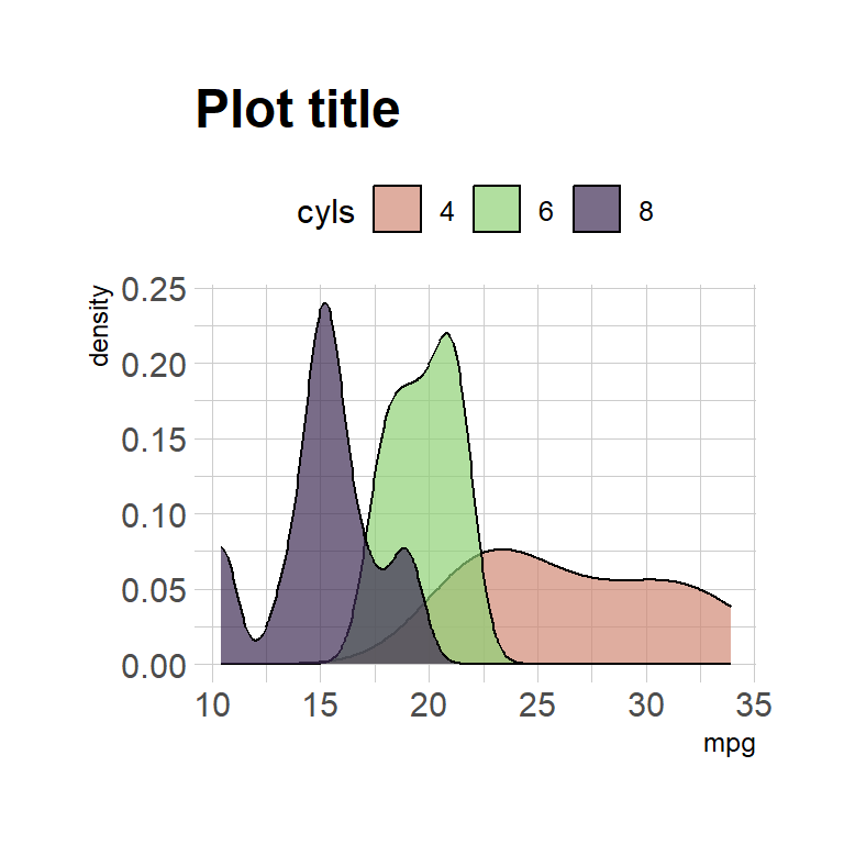
ggtitle("Plot title") +
theme_ipsum() + # Arial Narrow
scale_fill_ipsum() +
theme(legend.position = "top")library(ggplot2)
library(hrbrthemes)
cyls <- as.factor(mtcars$cyl)
ggplot(mtcars, aes(x = mpg, fill = cyls)) +
geom_density(alpha = 0.7) +
ggtitle("Plot title") +
theme_ipsum_es() + # Econ Sans Condensed
theme(legend.position = "top")library(ggplot2)
library(hrbrthemes)
cyls <- as.factor(mtcars$cyl)
ggplot(mtcars, aes(x = mpg, fill = cyls)) +
geom_density(alpha = 0.7) +
ggtitle("Plot title") +
theme_ipsum_rc() + # Roboto Condensed
theme(legend.position = "top")library(ggplot2)
library(hrbrthemes)
cyls <- as.factor(mtcars$cyl)
ggplot(mtcars, aes(x = mpg, fill = cyls)) +
geom_density(alpha = 0.7) +
ggtitle("Plot title") +
theme_ipsum_ps() + # IBM Plex Sans font
theme(legend.position = "top")library(ggplot2)
library(hrbrthemes)
cyls <- as.factor(mtcars$cyl)
ggplot(mtcars, aes(x = mpg, fill = cyls)) +
geom_density(alpha = 0.7) +
ggtitle("Plot title") +
theme_ipsum_pub() + # Public Sans
theme(legend.position = "top")library(ggplot2)
library(hrbrthemes)
cyls <- as.factor(mtcars$cyl)
ggplot(mtcars, aes(x = mpg, fill = cyls)) +
geom_density(alpha = 0.7) +
ggtitle("Plot title") +
theme_ipsum_tw() + # Titilium Web
theme(legend.position = "top")library(ggplot2)
library(hrbrthemes)
# import_roboto_condensed()
# extrafont::loadfonts(device="win")
cyls <- as.factor(mtcars$cyl)
ggplot(mtcars, aes(x = mpg, fill = cyls)) +
geom_density(alpha = 0.7) +
ggtitle("Plot title") +
theme_modern_rc() + # Roboto Condensed dark theme
theme(legend.position = "top")library(ggplot2)
library(hrbrthemes)
# import_roboto_condensed()
# extrafont::loadfonts(device="win")
cyls <- as.factor(mtcars$cyl)
ggplot(mtcars, aes(x = mpg, fill = cyls)) +
geom_density(alpha = 0.7) +
ggtitle("Plot title") +
theme_ft_rc() + # Dark theme based on FT’s dark theme
scale_fill_ft() +
theme(legend.position = "top")
ggthemr package
library(ggplot2)
library(ggthemr)

cyls <- as.factor(mtcars$cyl)

ggthemr("flat")

ggplot(mtcars, aes(x = mpg, fill = cyls)) +
  geom_density(alpha = 0.7) +
  theme(legend.position = "top")
library(ggplot2)
library(ggthemr)
cyls <- as.factor(mtcars$cyl)
ggthemr("flat dark")
ggplot(mtcars, aes(x = mpg, fill = cyls)) +
geom_density(alpha = 0.7) +
theme(legend.position = "top")library(ggplot2)
library(ggthemr)
cyls <- as.factor(mtcars$cyl)
ggthemr("camouflage")
ggplot(mtcars, aes(x = mpg, fill = cyls)) +
geom_density(alpha = 0.7) +
theme(legend.position = "top")library(ggplot2)
library(ggthemr)
cyls <- as.factor(mtcars$cyl)
ggthemr("carrot")
ggplot(mtcars, aes(x = mpg, fill = cyls)) +
geom_density(alpha = 0.7) +
theme(legend.position = "top")library(ggplot2)
library(ggthemr)
cyls <- as.factor(mtcars$cyl)
ggthemr("chalk")
ggplot(mtcars, aes(x = mpg, fill = cyls)) +
geom_density(alpha = 0.7) +
theme(legend.position = "top")library(ggplot2)
library(ggthemr)
cyls <- as.factor(mtcars$cyl)
ggthemr("copper")
ggplot(mtcars, aes(x = mpg, fill = cyls)) +
geom_density(alpha = 0.7) +
theme(legend.position = "top")library(ggplot2)
library(ggthemr)
cyls <- as.factor(mtcars$cyl)
ggthemr("dust")
ggplot(mtcars, aes(x = mpg, fill = cyls)) +
geom_density(alpha = 0.7) +
theme(legend.position = "top")library(ggplot2)
library(ggthemr)
cyls <- as.factor(mtcars$cyl)
ggthemr("earth")
ggplot(mtcars, aes(x = mpg, fill = cyls)) +
geom_density(alpha = 0.7) +
theme(legend.position = "top")library(ggplot2)
library(ggthemr)
cyls <- as.factor(mtcars$cyl)
ggthemr("freshe")
ggplot(mtcars, aes(x = mpg, fill = cyls)) +
geom_density(alpha = 0.7) +
theme(legend.position = "top")library(ggplot2)
library(ggthemr)
cyls <- as.factor(mtcars$cyl)
ggthemr("grape")
ggplot(mtcars, aes(x = mpg, fill = cyls)) +
geom_density(alpha = 0.7) +
theme(legend.position = "top")library(ggplot2)
library(ggthemr)
cyls <- as.factor(mtcars$cyl)
ggthemr("grass")
ggplot(mtcars, aes(x = mpg, fill = cyls)) +
geom_density(alpha = 0.7) +
theme(legend.position = "top")library(ggplot2)
library(ggthemr)
cyls <- as.factor(mtcars$cyl)
ggthemr("greyscale")
ggplot(mtcars, aes(x = mpg, fill = cyls)) +
geom_density(alpha = 0.7) +
theme(legend.position = "top")library(ggplot2)
library(ggthemr)
cyls <- as.factor(mtcars$cyl)
ggthemr("light")
ggplot(mtcars, aes(x = mpg, fill = cyls)) +
geom_density(alpha = 0.7) +
theme(legend.position = "top")library(ggplot2)
library(ggthemr)
cyls <- as.factor(mtcars$cyl)
ggthemr("lilac")
ggplot(mtcars, aes(x = mpg, fill = cyls)) +
geom_density(alpha = 0.7) +
theme(legend.position = "top")library(ggplot2)
library(ggthemr)
cyls <- as.factor(mtcars$cyl)
ggthemr("pale")
ggplot(mtcars, aes(x = mpg, fill = cyls)) +
geom_density(alpha = 0.7) +
theme(legend.position = "top")library(ggplot2)
library(ggthemr)
cyls <- as.factor(mtcars$cyl)
ggthemr("sea")
ggplot(mtcars, aes(x = mpg, fill = cyls)) +
geom_density(alpha = 0.7) +
theme(legend.position = "top")library(ggplot2)
library(ggthemr)
cyls <- as.factor(mtcars$cyl)
ggthemr("sky")
ggplot(mtcars, aes(x = mpg, fill = cyls)) +
geom_density(alpha = 0.7) +
theme(legend.position = "top")library(ggplot2)
library(ggthemr)
cyls <- as.factor(mtcars$cyl)
ggthemr("solarized")
ggplot(mtcars, aes(x = mpg, fill = cyls)) +
geom_density(alpha = 0.7) +
theme(legend.position = "top")Note that you will need to call ggthemr_reset() to reset to the default ggplot2 theme.
The ggthemr package works different than the other packages. Instead of using the theme function and set a theme you can set a theme globally making use of the ggthemr function and passing the theme as string as argument.
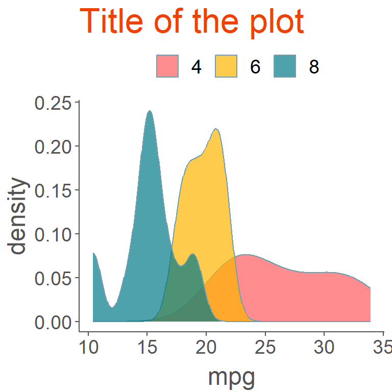
ggtech package
The ggtech package provides themes inspired by tech companies, such as Airbnb, Google, Twitter or Facebook.
library(ggplot2)
library(ggtech)

cyls <- as.factor(mtcars$cyl)

ggplot(mtcars, aes(x = mpg, fill = cyls)) +
  geom_density(alpha = 0.7) +
  ggtitle("Title of the plot") +
  theme_tech(theme = "airbnb") +
  scale_fill_tech(theme = "airbnb") +
  theme(legend.position = "top")
library(ggplot2)
library(ggtech)
cyls <- as.factor(mtcars$cyl)
ggplot(mtcars, aes(x = mpg, fill = cyls)) +
geom_density(alpha = 0.7) +
ggtitle("Title of the plot") +
theme_tech(theme = "etsy") +
scale_fill_tech(theme = "etsy") +
theme(legend.position = "top")library(ggplot2)
library(ggtech)
cyls <- as.factor(mtcars$cyl)
ggplot(mtcars, aes(x = mpg, fill = cyls)) +
geom_density(alpha = 0.7) +
ggtitle("Title of the plot") +
theme_tech(theme = "facebook") +
scale_fill_tech(theme = "facebook") +
theme(legend.position = "top")library(ggplot2)
library(ggtech)
cyls <- as.factor(mtcars$cyl)
ggplot(mtcars, aes(x = mpg, fill = cyls)) +
geom_density(alpha = 0.7) +
ggtitle("Title of the plot") +
theme_tech(theme = "google") +
scale_fill_tech(theme = "google") +
theme(legend.position = "top")library(ggplot2)
library(ggtech)
cyls <- as.factor(mtcars$cyl)
ggplot(mtcars, aes(x = mpg, fill = cyls)) +
geom_density(alpha = 0.7) +
ggtitle("Title of the plot") +
theme_tech(theme = "twitter") +
scale_fill_tech(theme = "twitter") +
theme(legend.position = "top")library(ggplot2)
library(ggtech)
cyls <- as.factor(mtcars$cyl)
ggplot(mtcars, aes(x = mpg, fill = cyls)) +
geom_density(alpha = 0.7) +
ggtitle("Title of the plot") +
theme_airbnb_fancy() +
scale_fill_tech(theme = "airbnb") +
theme(legend.position = "top")
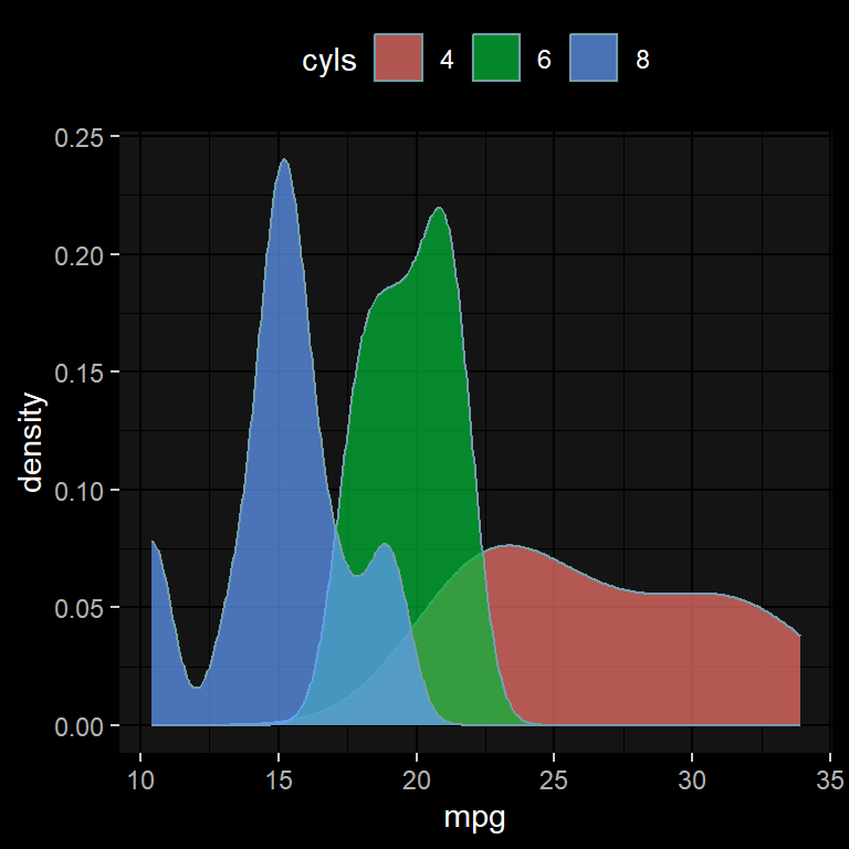
ggdark package
library(ggplot2)
library(ggdark)

cyls <- as.factor(mtcars$cyl)

ggplot(mtcars, aes(x = mpg, fill = cyls)) +
  geom_density(alpha = 0.7) +
  dark_theme_gray() +  # Default
  theme(legend.position = "top")
library(ggplot2)
library(ggdark)
cyls <- as.factor(mtcars$cyl)
ggplot(mtcars, aes(x = mpg, fill = cyls)) +
geom_density(alpha = 0.7) +
dark_theme_bw() +
theme(legend.position = "top")library(ggplot2)
library(ggdark)
cyls <- as.factor(mtcars$cyl)
ggplot(mtcars, aes(x = mpg, fill = cyls)) +
geom_density(alpha = 0.7) +
dark_theme_linedraw() +
theme(legend.position = "top")library(ggplot2)
library(ggdark)
cyls <- as.factor(mtcars$cyl)
ggplot(mtcars, aes(x = mpg, fill = cyls)) +
geom_density(alpha = 0.7) +
dark_theme_light() +
theme(legend.position = "top")library(ggplot2)
library(ggdark)
cyls <- as.factor(mtcars$cyl)
ggplot(mtcars, aes(x = mpg, fill = cyls)) +
geom_density(alpha = 0.7) +
dark_theme_dark() +
theme(legend.position = "top")library(ggplot2)
library(ggdark)
cyls <- as.factor(mtcars$cyl)
ggplot(mtcars, aes(x = mpg, fill = cyls)) +
geom_density(alpha = 0.7) +
dark_theme_minimal() +
theme(legend.position = "top")library(ggplot2)
library(ggdark)
cyls <- as.factor(mtcars$cyl)
ggplot(mtcars, aes(x = mpg, fill = cyls)) +
geom_density(alpha = 0.7) +
dark_theme_classic() +
theme(legend.position = "top")library(ggplot2)
library(ggdark)
cyls <- as.factor(mtcars$cyl)
ggplot(mtcars, aes(x = mpg, fill = cyls)) +
geom_density(alpha = 0.7) +
dark_theme_void() +
theme(legend.position = "top")library(ggplot2)
library(ggdark)
library(ggthemes)
cyls <- as.factor(mtcars$cyl)
invert_geom_defaults()
ggplot(mtcars, aes(x = mpg, fill = cyls)) +
geom_density(alpha = 0.7) +
dark_mode(theme_solarized()) +
scale_fill_solarized() +
theme(legend.position = "top")
invert_geom_defaults()ggdark provides the dark mode themes of the in-built ggplot2 themes. In addition, the package can convert any theme into a dark theme making use of the dark_mode function.
Set an active theme
The theme_set function can be used to set a theme globally. In the following example we are setting the in-built theme_dark to all the generated plots. Then, you can you back to the default theme as follows.
library(ggplot2)

# Global theme
old <- theme_set(theme_dark())

cyls <- as.factor(mtcars$cyl)

ggplot(mtcars, aes(x = mpg, fill = cyls)) +
  geom_density(alpha = 0.7) +
  theme(legend.position = "top")

# Reset to default
theme_set(old)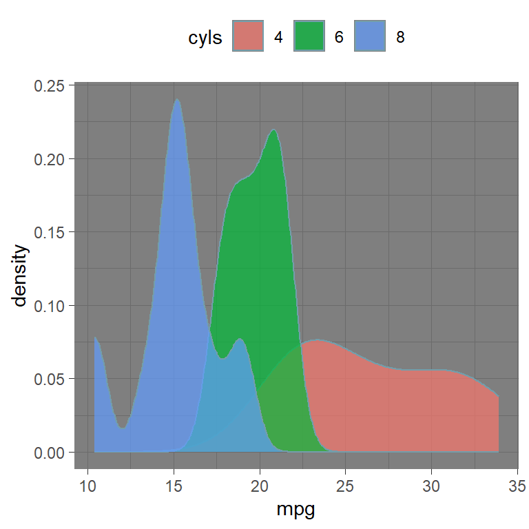

Master Statistics
Learn statistics from the basics to advanced techniques, clearly explained
Go to site