Simple plot combination: mfrow and mfcol
It is straightforward to combine plots in base R with mfrow and mfcol graphical parameters. You just need to specify a vector with the number of rows and the number of columns you want to create. The decision of which graphical parameter you should use depends on how do you want your plots to be arranged:
mfrow: the plots will be arranged by rows.mfcol: the plots will be arranged by columns.
As an example, if you want to combine two plots you just need to type the following:
# Data
x <- rexp(50)

# One row, two columns
par(mfrow = c(1, 2))

# The following two plots will be combined
hist(x, main = "Left plot")     # Left
boxplot(x, main = "Right plot") # Right

# Back to the original graphics device
par(mfrow = c(1, 1))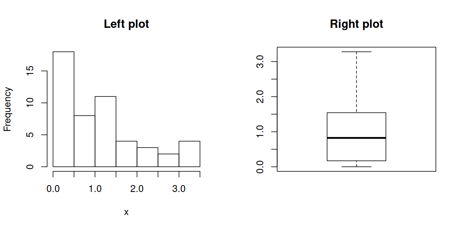
If you need to add more rows, modify the vector:
# Data
set.seed(6)
x <- rexp(50)
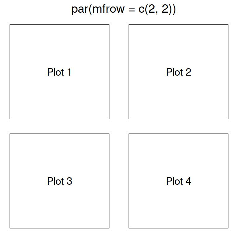
# Two rows, two columns
par(mfrow = c(2, 2))
# Plots
hist(x, main = "Top left") # Top left
boxplot(x, main = "Top right") # Top right
plot(x, main = "Bottom left") # Bottom left
pie(table(round(x)), main = "Bottom right") # Bottom right
# Back to the original graphics device
par(mfrow = c(1, 1))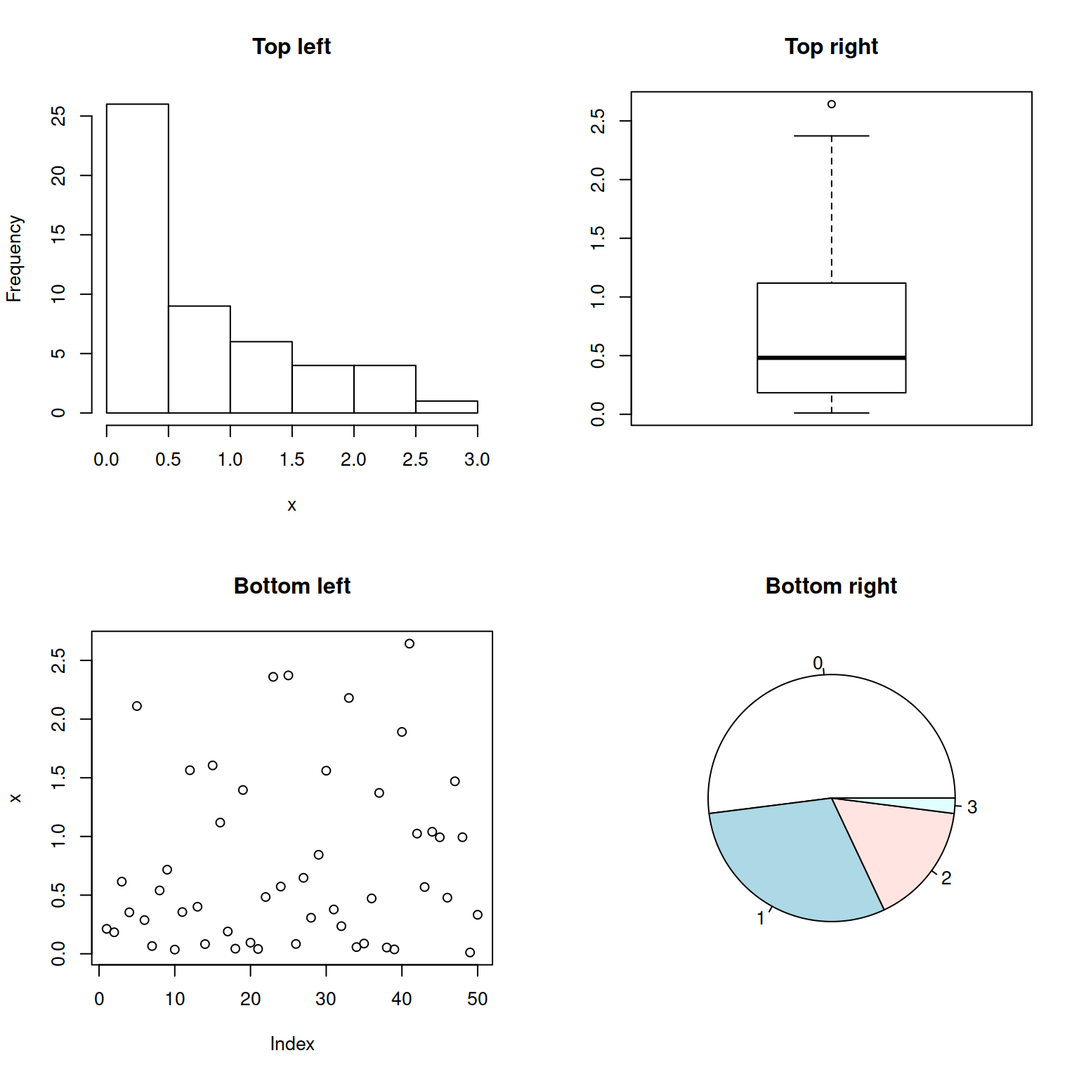
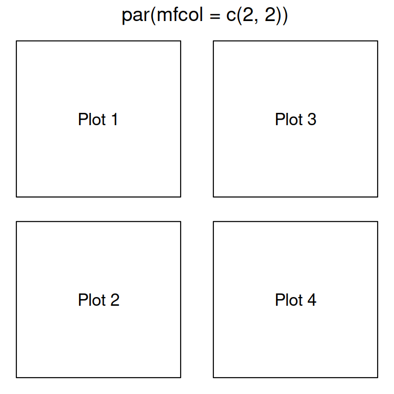
If you prefer your plots to be arranged by column, use the mfcol graphical parameter instead:
# Data
set.seed(6)
x <- rexp(50)

# Two rows, two columns
par(mfcol = c(2, 2))

# Plots
hist(x, main = "Top left")                   # Top left
boxplot(x, main = "Bottom left")             # Bottom left
plot(x, main = "Top right")                  # Top right
pie(table(round(x)), main = "Bottom right")  # Bottom right

# Back to the original graphics device
par(mfcol = c(1, 1))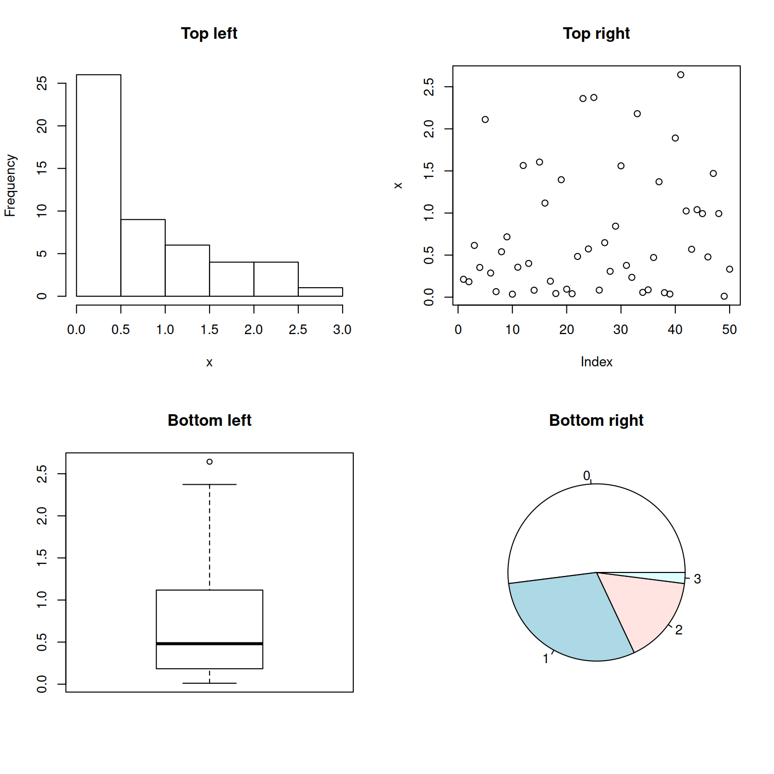
Complex layouts: layout function
In case you need more complex layouts you can use the layout function. The arguments of the function are the following:
mat: a matrix where each value represents the location of the figures.widths: a vector for the widths of the columns. You can also specify them in centimeters withlcmfunction.heights: a vector for the height of the columns. You can also specify them in centimeters withlcmfunction.respect: Boolean or a matrix filled with 0 and 1 of the same dimensions asmatto indicate whether to respect relations between widths and heights or not.
Note that you can preview a layout making use of the layout.show function before adding the plots.
l <- layout(matrix(c(1, 2,  # First, second
                     3, 3), # and third plot
            nrow = 2,
            ncol = 2,
            byrow = TRUE))

layout.show(l)
Example 1: two rows, with two plots on the first and one on the second.
Using the layout we created before, you can add the plots as follows.
mat <- matrix(c(1, 2,  # First, second
                3, 3), # and third plot
              nrow = 2, ncol = 2,
              byrow = TRUE)

layout(mat = mat)

# Data
set.seed(6)
x <- rexp(50)

plot(x)    # First plot
boxplot(x) # Second plot
hist(x)    # Third plot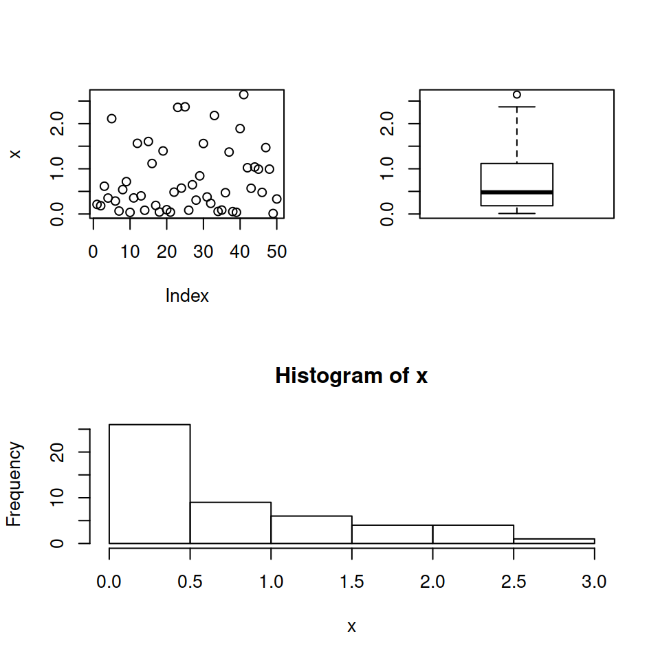
Example 2: two rows, with two plots below and one above, being the second row three times higher than the first.
mat <- matrix(c(1, 1,  # First
                2, 3), # second and third plot
              nrow = 2, ncol = 2,
              byrow = TRUE)

layout(mat = mat,
       heights = c(1, 3)) # First and second row
                          # relative heights

# Data
set.seed(6)
x <- rexp(50)

plot(x)    # First row
boxplot(x) # Second row, left
hist(x)    # Second row, right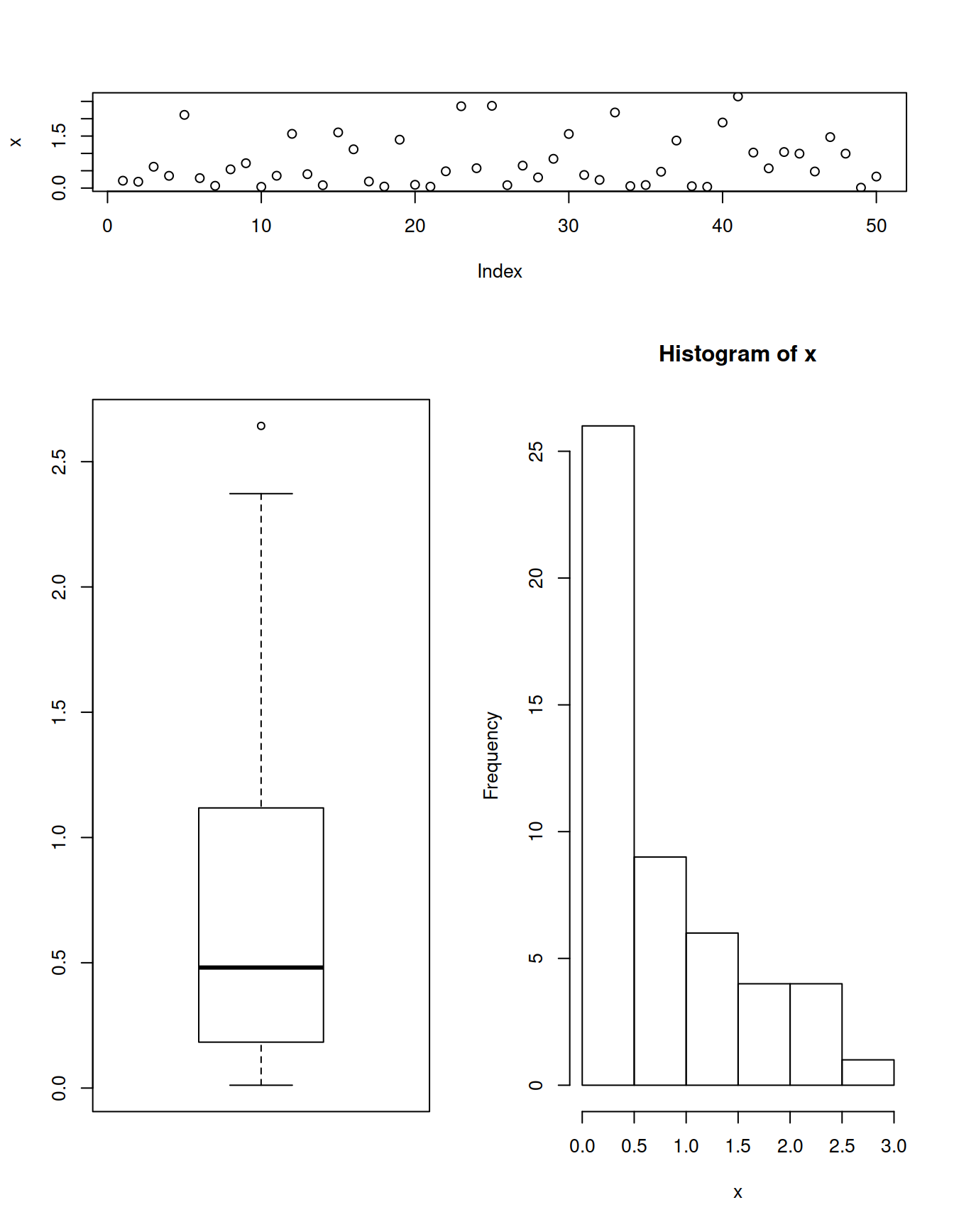
Example 3: two columns, with two plots on the right and one on the left, being the second column two times wider than de first.
mat <- matrix(c(1, 2,  # First, second
                1, 3), # first and third plot
              nrow = 2, ncol = 2,
              byrow = TRUE),

layout(mat = mat,
       widths = c(1, 2)) # First and second
                         # column relative widths

# Data
set.seed(6)
x <- rexp(50)

plot(x)    # First column, top
boxplot(x) # First column, bottom
hist(x)    # Second column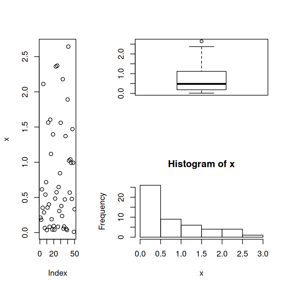
Marginal plots
With the layout function you can also add marginal plots to a plot. For that you could do something like the following. Note that you will need to customize several graphical parameters for each plot.
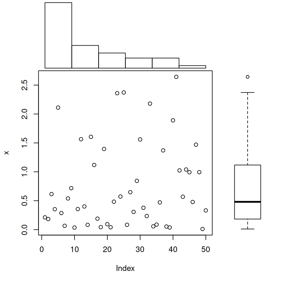
# Data
set.seed(6)
x <- rexp(50)

layout(matrix(c(2, 0, 1, 3),
              nrow = 2, ncol = 2,
              byrow = TRUE),
       widths = c(3, 1),
       heights  = c(1, 3), respect = TRUE)

# Top and right margin of the main plot
par(mar = c(5.1, 4.1, 0, 0))
plot(x)

# Left margin of the histogram
par(mar = c(0, 4.1, 0, 0))
hist(x, main = "", bty = "n",
     axes = FALSE, ylab = "")

# Bottom margin of the boxplot
par(mar = c(5.1, 0, 0, 0))

# Boxplot without plot region box
par(bty = "n")

# Boxplot without axes
boxplot(x, axes = FALSE)
Master Statistics
Learn statistics from the basics to advanced techniques, clearly explained
Go to site