The legend function allows adding legends to base R plots.
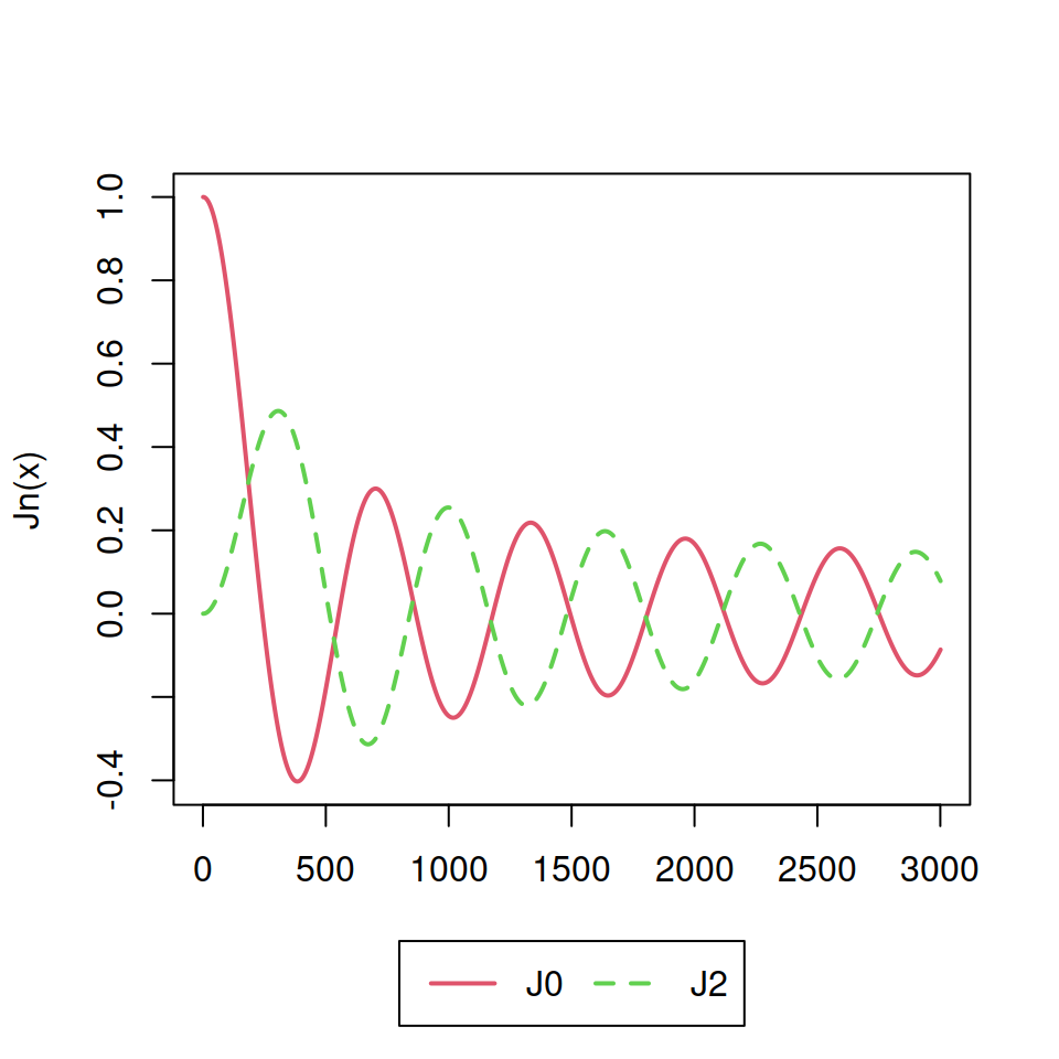
We are going to use the following plot on the examples of this guide.
# Reproducible plot
plotl <- function(points = FALSE, ...) {
    x <- seq(0, 30, 0.01)
    plot(besselJ(x, 0), col = 2, type = "l",
         lwd = 2, ylab = "Jn(x)", xlab = "", ...)
    lines(besselJ(x, 2), col = 3,
          type = "l", lwd = 2, lty = 2)
    if(points == TRUE) {
      points(c(1335, 1325),
             c(besselJ(x, 0)[1335],
               besselJ(x, 2)[1325]),
             pch = c(15, 18), cex = 2, col = 2:3)
    }
}

plotl()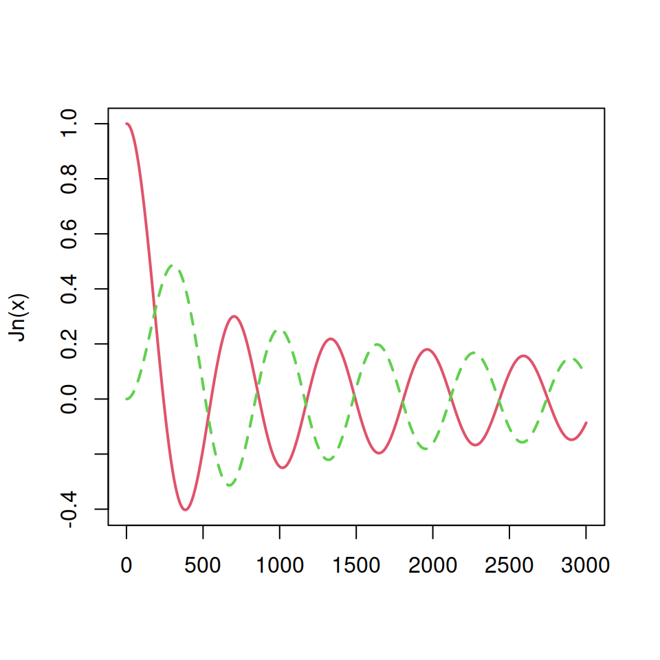
Legend position, lines and fill
Option 1. Set the argument x to "top", "topleft", "topright", "bottom", "bottomleft", "bottomright", "left", "right" or "center". In this scenario you don’t have to set the argument y.
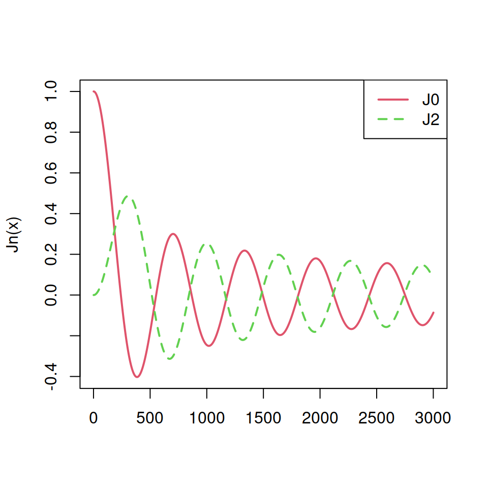
The text of the legend can be set with legend argument and the line type, width and color with lty, lwd and col arguments, respectively.
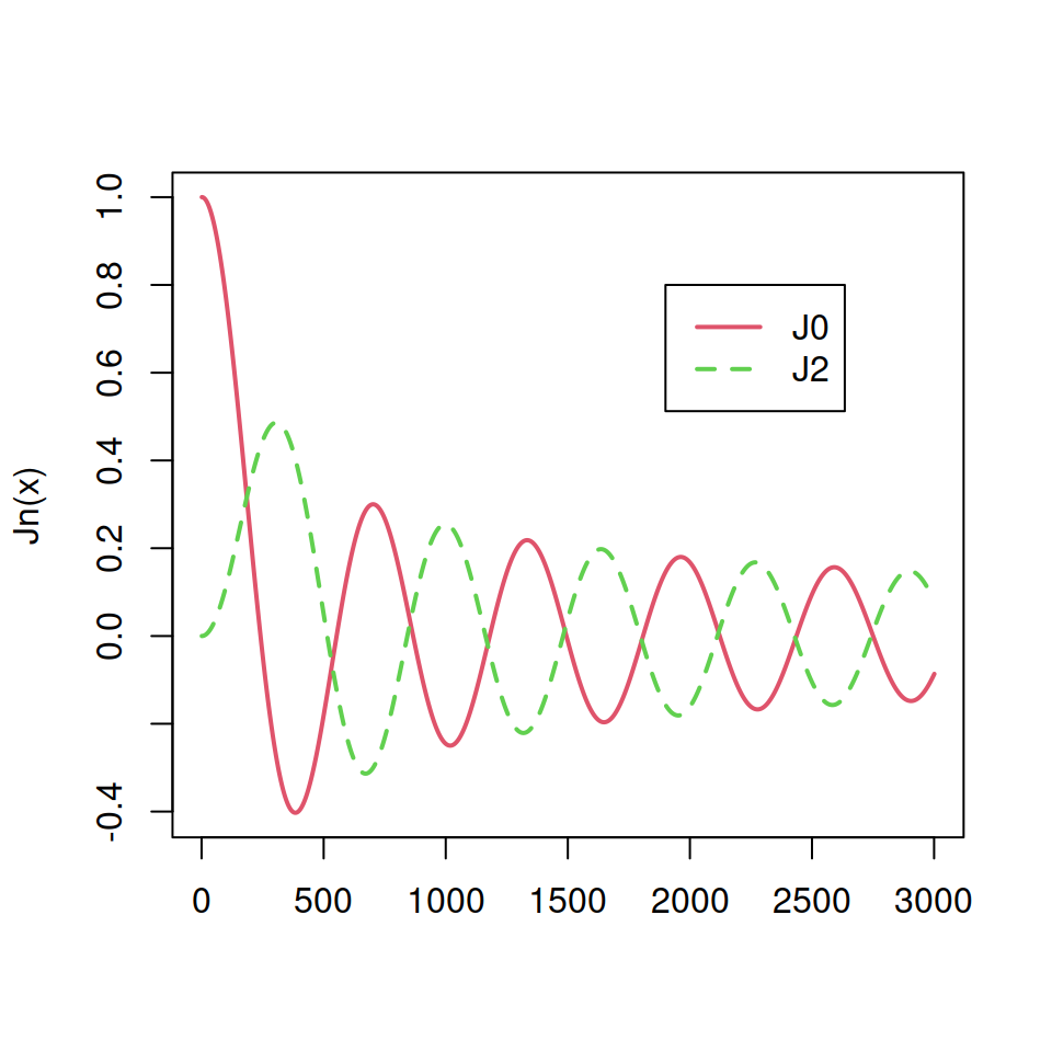
plotl()
legend(x = "topright",         # Position
       legend = c("J0", "J2"), # Legend texts
       lty = c(1, 2),          # Line types
       col = c(2, 3),          # Line colors
       lwd = 2)                # Line widths
Option 2. Use the arguments x and y as coordinates to indicate where to draw the legend.
plotl()
legend(x = 1900, y = 0.8,      # Coordinates
       legend = c("J0", "J2"), # Legend texts
       lty = c(1, 2),          # Line types
       col = c(2, 3),          # Line colors
       lwd = 2)                # Line widths
Option 3. Use a position and specify a margin from the border with the inset argument.
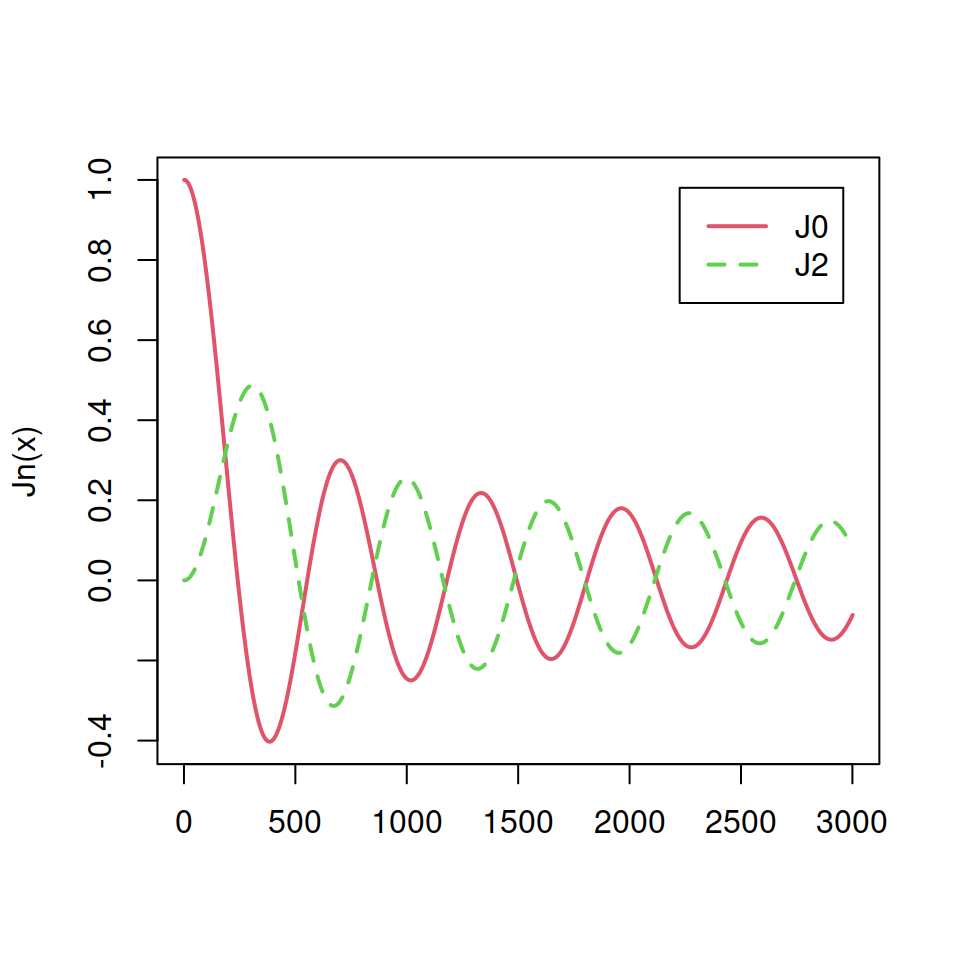
The value of the argument represents the distance from the margin as a fraction of the plot region.
plotl()
legend("topright",
       inset = 0.05, # Distance from the margin
       legend = c("J0", "J2"),
       lty = c(1, 2),
       col = c(2, 3),
       lwd = 2)
Note that you can also set pch symbols over the legend lines if needed.
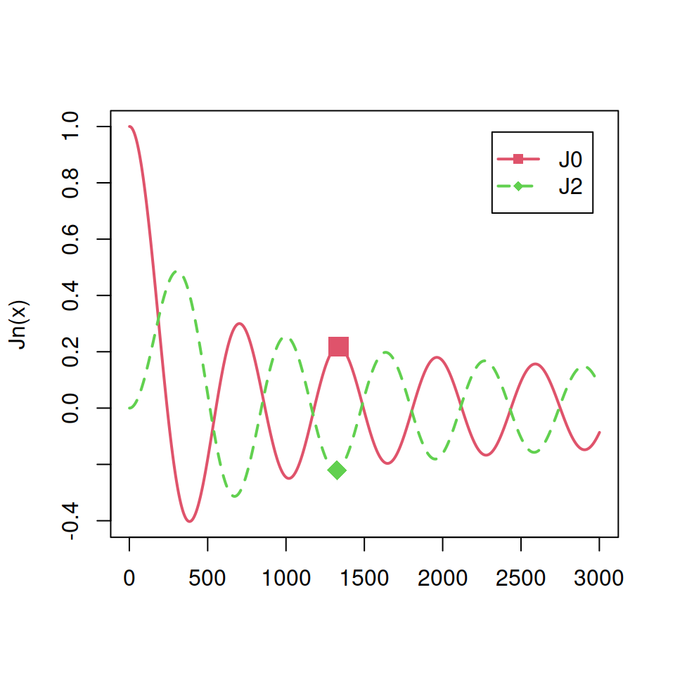
plotl(points = TRUE)
legend("topright",
       inset = 0.05,
       legend = c("J0", "J2"),
       lty = c(1, 2),
       col = c(2, 3),
       lwd = 2,
       pch = c(15, 18)) # pch symbols
If you have a bar plot, pie chart or any other filled plot you can set the argument fill instead of lty.
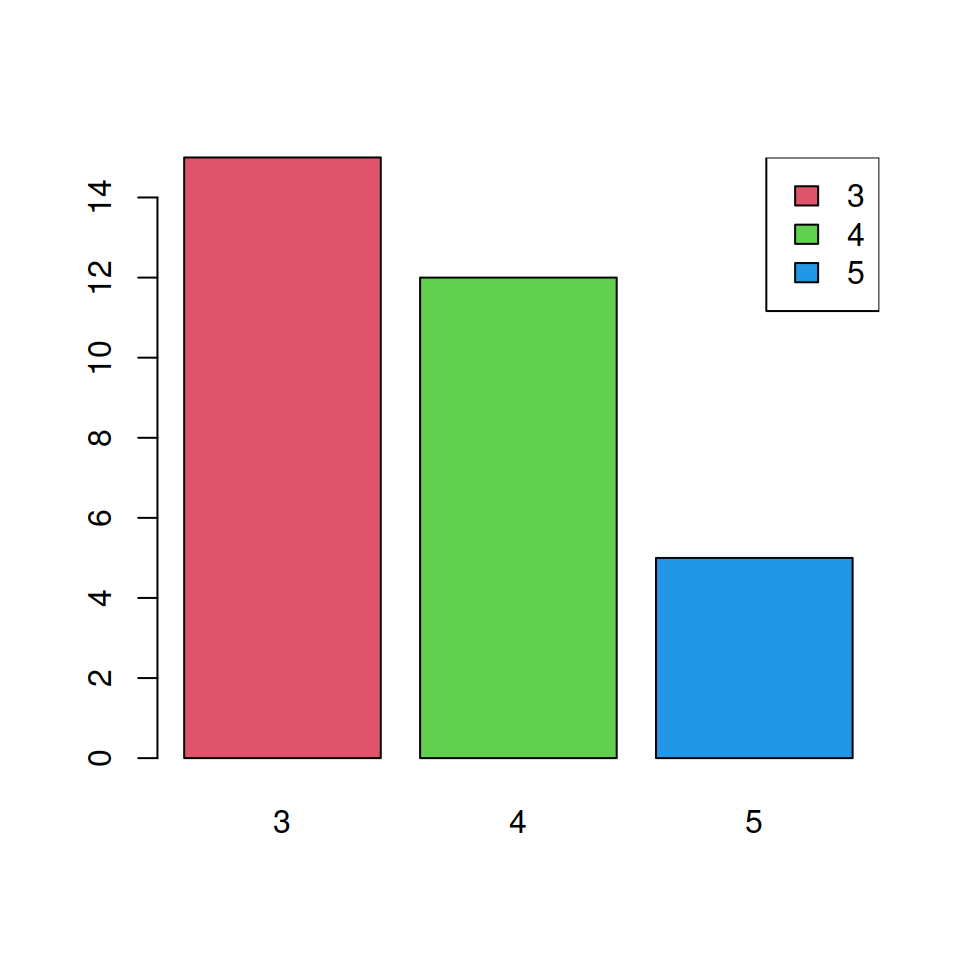
You can create filled squares with the fill argument, which border color can be modified with the border argument.
barplot(table(mtcars$gear), col = 2:4)

legend("topright",
       legend = c(3, 4, 5),
       fill = 2:4,       # Color of the squares
       border = "black") # Color of the border
                         # of the squares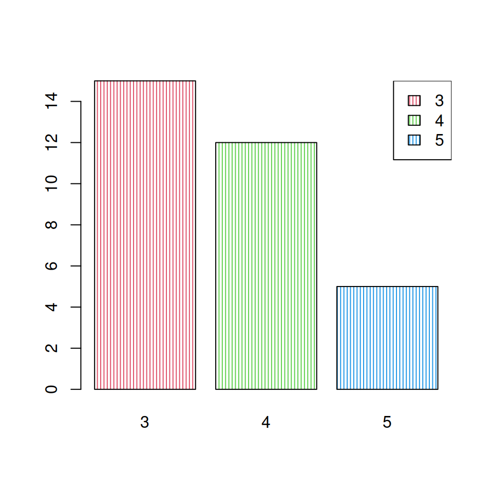
If the areas of your plot are shaded you can specify the density and angle arguments to match them.
barplot(table(mtcars$gear), col = 2:4,
        density = 30, angle = 90)

legend("topright",
       legend = c(3, 4, 5),
       fill = 2:4,
       density = 30, # Shading lines density
       angle = 90)   # Angle of the shading lines
Legend orientation
Setting horiz = FALSE will display the legend in landscape mode.
plotl()
legend("top",
       legend = c("J0", "J2"),
       lty = c(1, 2),
       col = c(2, 3),
       lwd = 2,
       horiz = TRUE)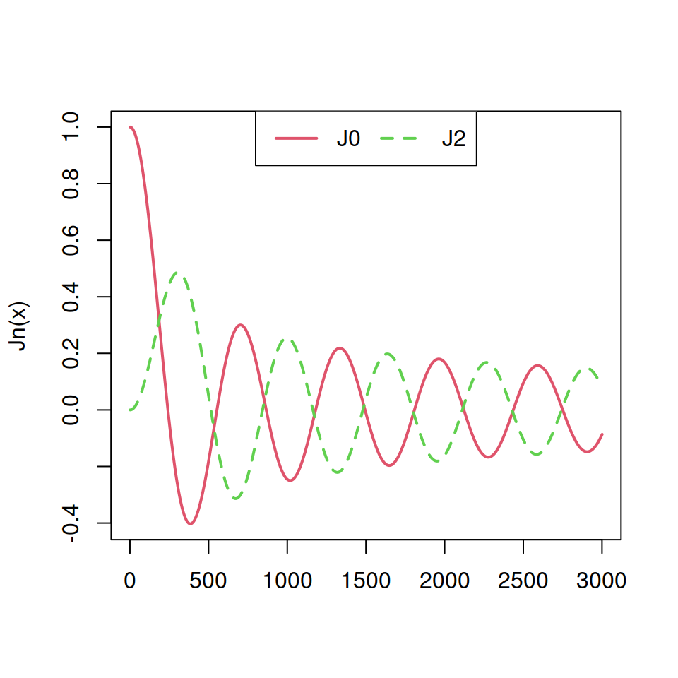
You can also specify the number of columns of the legend if horiz = FALSE with the argument ncol.
plotl()
legend("top",
       legend = c("J0", "J2"),
       lty = c(1, 2),
       col = c(2, 3),
       lwd = 2,
       ncol = 2)
Legend title
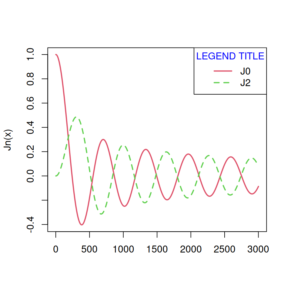
It is possible to add a title to a legend and modify its horizontal adjustment and color with the title, title.adj and title.col arguments, respectively.
plotl()
legend("topright", legend = c("J0", "J2"),
       title = "LEGEND TITLE",  # Title
       title.adj = 0.5,    # Horizontal adjustment
       title.col = "blue", # Color of the title
       lty = c(1, 2), col = c(2, 3), lwd = 2)
Box border and background color of the legend
The box.lty, box.lwd and box.col arguments allows modifying the line type, width and color of the legend box, respectively.
plotl()
legend(1500, 0.9,
       legend = c("J0", "J2"),
       box.lty = 2, # Line type of the box
       box.lwd = 2, # Box line width
       box.col = 4, # Box line color
       lty = c(1, 2),
       col = c(2, 3),
       lwd = 2)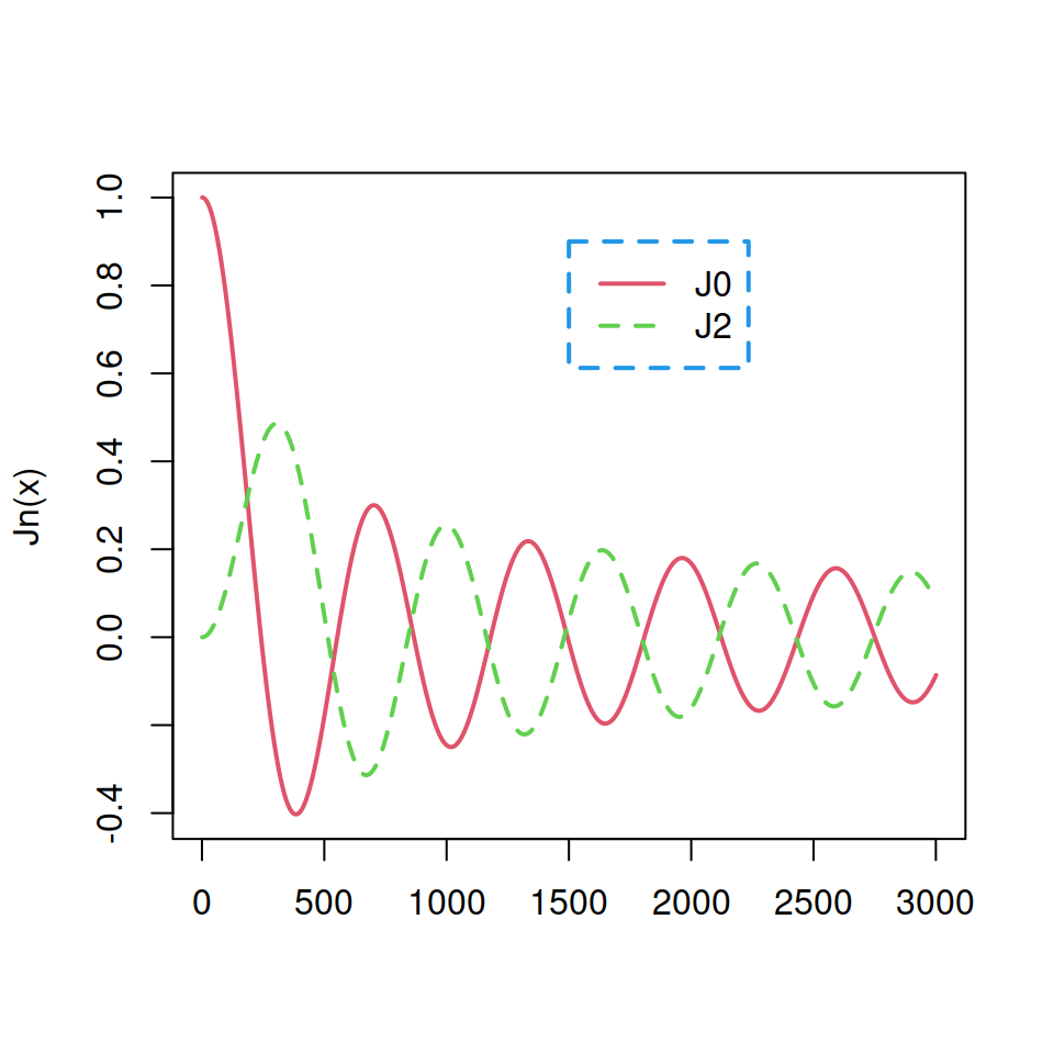
In addition to the previous you can also modify the background color of the box with the bg argument.
plotl()
legend("topright", inset = 0.05,
       legend = c("J0", "J2"),
       bg = rgb(1, 0, 0, alpha = 0.15),
       lty = c(1, 2),
       col = c(2, 3),
       lwd = 2)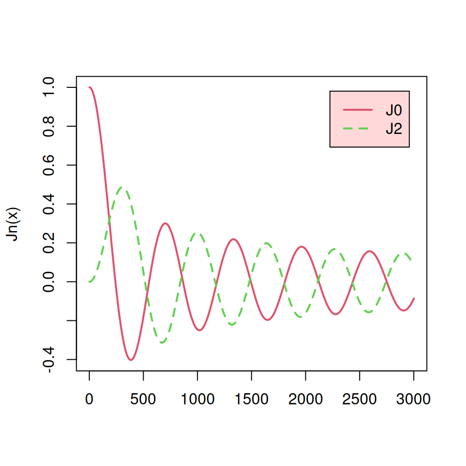
Remove legend box
You can remove the box of the legend by two different methods.
Option 1. Set bty = "n".
plotl()
legend(1500, 0.9,
       legend = c("J0", "J2"),
       bty = "n", # Removes the legend box
       lty = c(1, 2),
       col = c(2, 3),
       lwd = 2)
Option 2. Set box.lty = 0
plotl()
legend(1500, 0.9,
       legend = c("J0", "J2"),
       box.lty = 0, # Removes the box line
       lty = c(1, 2),
       col = c(2, 3),
       lwd = 2)
Legend size
The cex argument controls the size of the legend. The default value is 1.
plotl()
legend("topright",
       legend = c("J0", "J2"),
       lty = c(1, 2),
       col = c(2, 3),
       cex = 1.5, # Legend size
       lwd = 2)
Legend outside the plot
In some scenarios you will need to set the legend outside of the plot because it doesn’t fit inside. For that purpose you will need to increase the margins of the plot, set the legend, use xpd = TRUE and fine tune the values of the inset argument.
# Make the window wider than taller
# windows(width = 5.5, height = 5)

# Save current graphical parameters
opar <- par(no.readonly = TRUE)

# Change the margins of the plot
# (the fourth is the right margin)
par(mar = c(6, 5, 4, 6.5))

plotl()
legend(x = "topright",
       inset = c(-0.35, 0), # You will need to fine-tune the first
                            # value depending on the windows size
       legend = c("J0", "J2"),
       lty = c(1, 2),
       col = c(2, 3),
       lwd = 2,
       xpd = TRUE) # Needed to put the legend outside the plot

# Back to the default graphical parameters
on.exit(par(opar))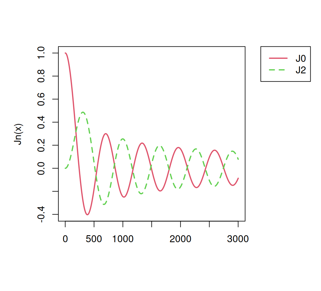
Legend under the plot
An alternative is to set the legend below (or above) the plot following the same approach we followed before but increasing the bottom or upper margins.
# windows(width = 5, height = 5)

# Save current graphical parameters
opar <- par(no.readonly = TRUE)

# Change the margins of the plot (the first is the bottom margin)
par(mar = c(6, 4.1, 4.1, 2.1))

plotl()
legend(x = "bottom",
       inset = c(0, -0.35), # You will need to fine-tune the second
                            # value depending on the windows size
       legend = c("J0", "J2"),
       lty = c(1, 2),
       col = c(2, 3),
       lwd = 2,
       xpd = TRUE, # You need to specify this graphical parameter to add
                   # the legend outside the plot area
       horiz = TRUE) # Horizontal legend

# Back to the default graphical parameters
on.exit(par(opar))