Anatogram images in ggplot2 with gganatogram

Package

Author

Jesper Maag

Human anatogram plot

The gganatogram function of the package of the same name can be used to create anatogram atlases. The package comes with four data sets: hgMale_key, hgMale_key, cell_key and other_key. Note that you can also create your own data frame.

Male

In order to create a male anatogram pass the hgMale_key data frame to the gganatogram function, specify organism = "human" and sex = "male". Note that we set a void theme and coord_fixed to maintain the aspect ratio.

# install.packages("remotes")
# remotes::install_github("jespermaag/gganatogram")
library(gganatogram)

gganatogram(data = hgMale_key,
            organism = "human", sex = "male",
            fill = "colour", fillOutline = "#a6bddb") +
  theme_void() + 
  coord_fixed()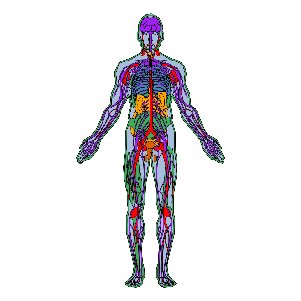

Male anatogram in ggplot2

Female

The process for creating a human female anatogram is analogous to the male anatogram, but passing the hgFemale_key data frame and specifying sex = "female".

# install.packages("remotes")
# remotes::install_github("jespermaag/gganatogram")
library(gganatogram)

gganatogram(data = hgFemale_key,
            organism = "human", sex = "female",
            fill = "colour", fillOutline = "#a6bddb") +
  theme_void() + 
  coord_fixed()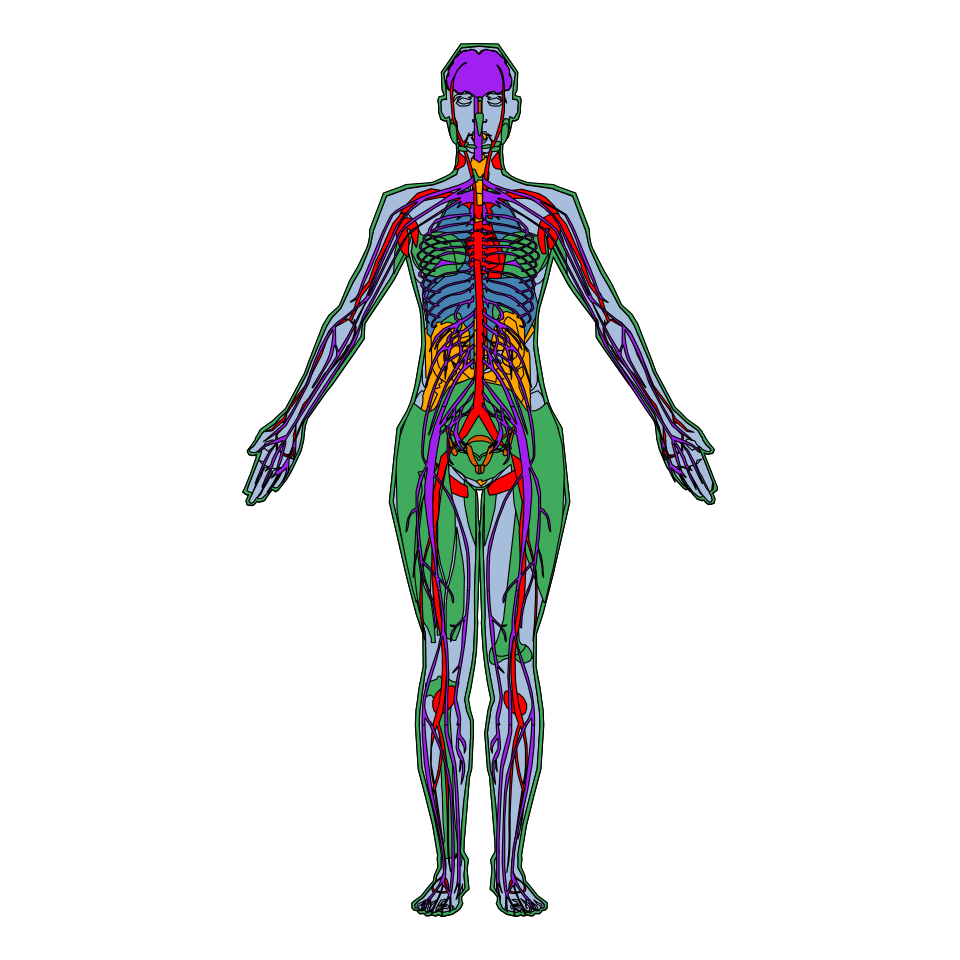

Female anatogram in ggplot2

Zoom

In case you need to make zoom to a specific part of the anatogram you can use coord_cartesian. Recall to remove the theme_void if you want to see the axes values.

# install.packages("remotes")
# remotes::install_github("jespermaag/gganatogram")
library(gganatogram)

gganatogram(data = hgMale_key,
            organism = "human", sex = "male",
            fill = "colour", fillOutline = "#a6bddb") +
  coord_cartesian(xlim = c(30, 75), ylim = c(-40, 0)) +
  theme_void()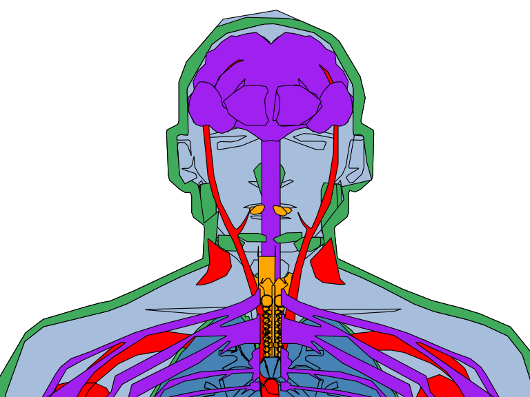

Anatogram zoom in R

Systems

The default plot displays all the body systems, but you can specify only some of them. You can also set outline = FALSE to only plot the systems. Type hgMale_key$type or hgFemale_key$type to see the available options.

# install.packages("remotes")
# remotes::install_github("jespermaag/gganatogram")
library(gganatogram)
# install.packages("dplyr")
library(dplyr)

hgMale_key %>%
  filter(type %in% "nervous_system") %>%
  gganatogram(organism = "human", sex = "male",
              fill = "colour", outline = FALSE) +
  theme_void() + 
  coord_fixed()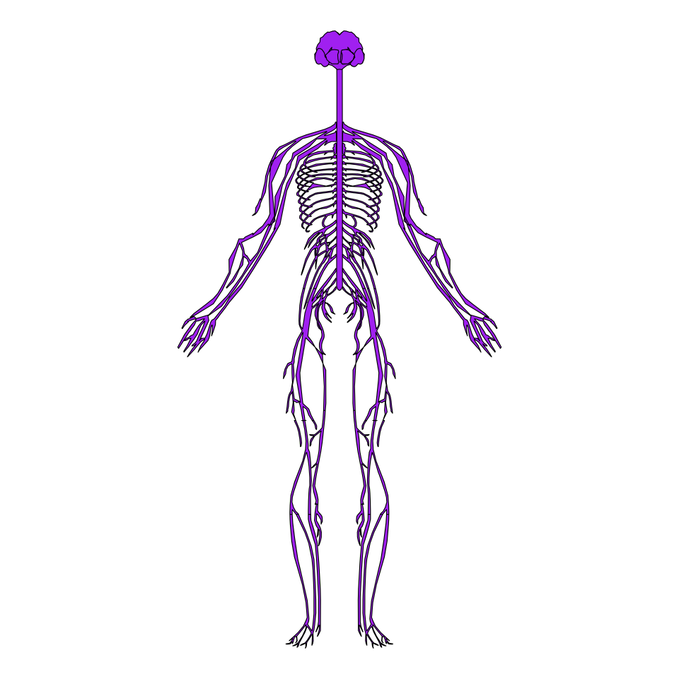

Anatogram systems in ggplot2

Organs

Similarly to plotting some systems you can plot only some organs. Type hgMale_key$organ or hgFemale_key$organ for a list containing the organ names.

# install.packages("remotes")
# remotes::install_github("jespermaag/gganatogram")
library(gganatogram)
# install.packages("dplyr")
library(dplyr)

hgMale_key %>%
  filter(organ %in% c("brain", "heart")) %>%
  gganatogram(organism = "human", sex = "male",
              fill = "colour") +
  theme_void() + 
  coord_fixed()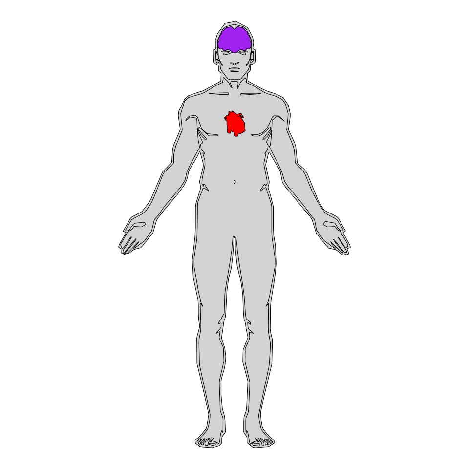

Displaying body organs plot

Color scale

The color scale can be customized based on the values column of the data frames and adding a continuous color scale, such as viridis.

# install.packages("remotes")
# remotes::install_github("jespermaag/gganatogram")
library(gganatogram)

gganatogram(data = hgMale_key,
            organism = "human", sex = "male",
            fill = "value",
            fillOutline = "#a6bddb") +
  theme_void() + 
  scale_fill_viridis_c() +
  coord_fixed()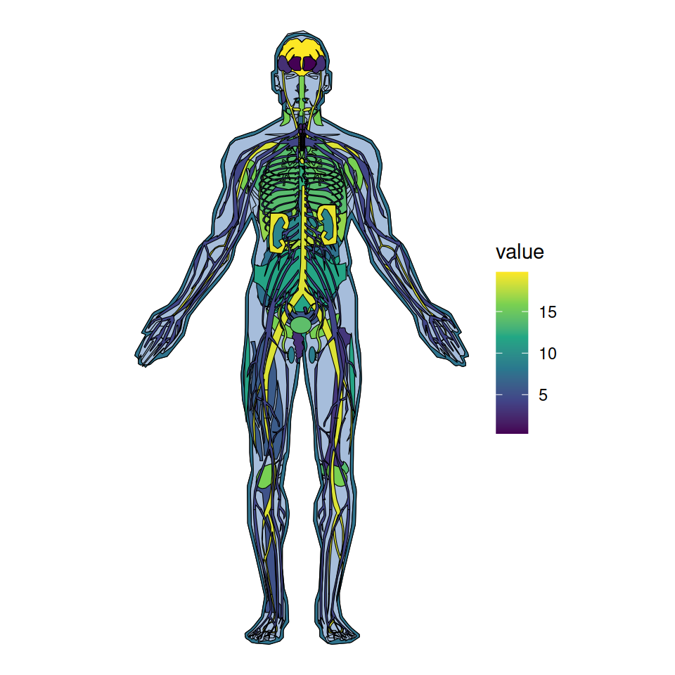

Anatogram in ggplot2 with viridis color scale

Other organisms

You can also specify more organisms, such as mice, cells and other animal species. Note that you can apply the same customization to the following anatograms that the ones described in the previous section.

Mouse anatogram in ggplot2

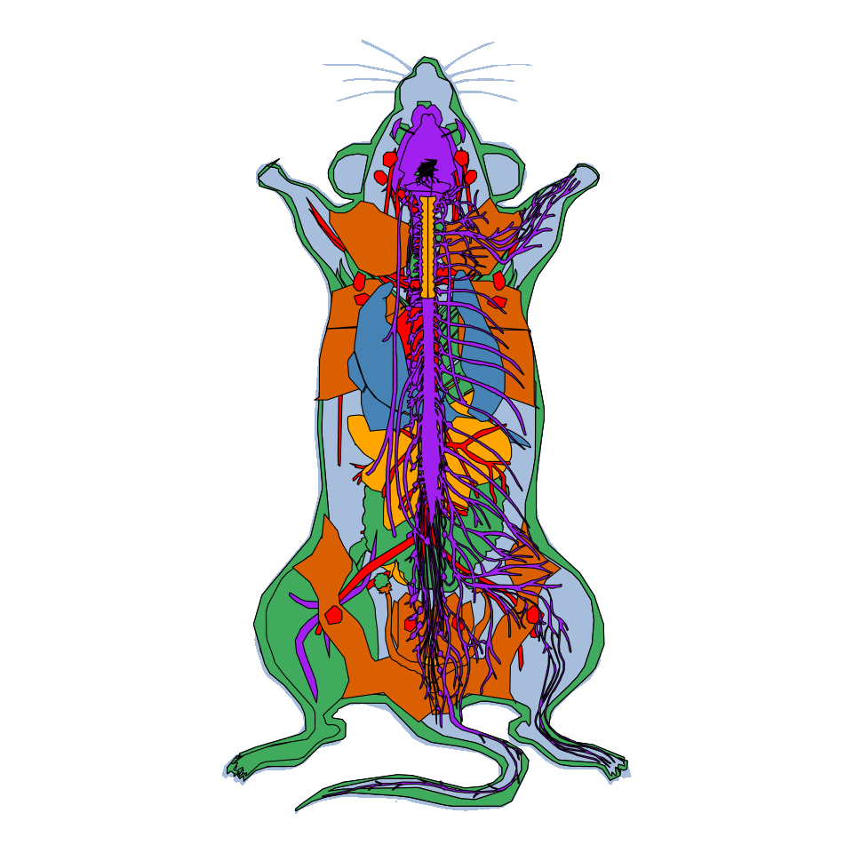
Mouse

# install.packages("remotes")
# remotes::install_github("jespermaag/gganatogram")
library(gganatogram)

gganatogram(data = mmFemale_key,
            organism = "mouse", sex = "female", 
            fillOutline = "#a6bddb", fill = "colour") +
  theme_void() +
  coord_fixed()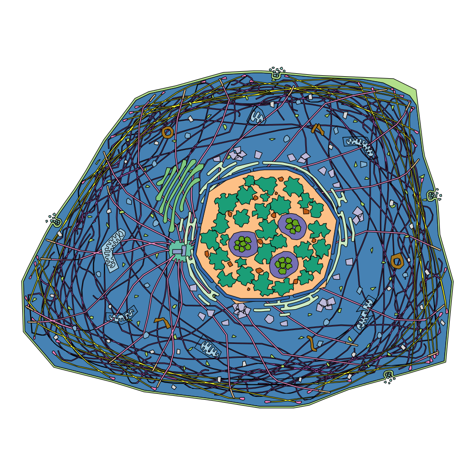

Cell plot in R ggplot2

Cell

# install.packages("remotes")
# remotes::install_github("jespermaag/gganatogram")
library(gganatogram)

gganatogram(data = cell_key$cell,
            organism = "cell",
            fillOutline = "#a6bddb", fill = "colour") +
  theme_void() +
  coord_fixed()

The other_key list contains 24 data frames with different organisms. In the following examples we selected some of them but recall that there are more options available to choose.

gganatogram R library

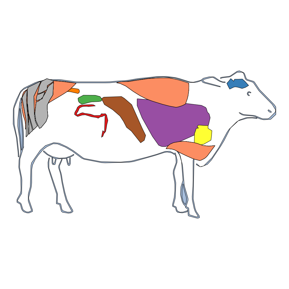
Taurus

# install.packages("remotes")
# remotes::install_github("jespermaag/gganatogram")
library(gganatogram)

gganatogram(data = other_key$bos_taurus,
            organism = "bos_taurus", sex = "male",
            fillOutline = "#a6bddb", fill = "colour") +
  theme_void() +
  coord_fixed()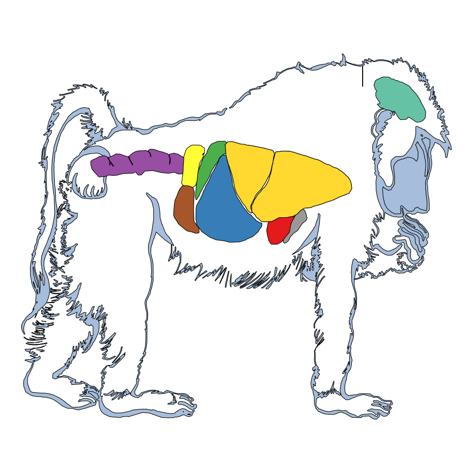

Plotting organisms with gganatogram

Papio Anubis

# install.packages("remotes")
# remotes::install_github("jespermaag/gganatogram")
library(gganatogram)

gganatogram(data = other_key$papio_anubis,
            organism = "papio_anubis", sex = "male",
            fillOutline = "#a6bddb", fill = "colour") +
  theme_void() +
  coord_fixed()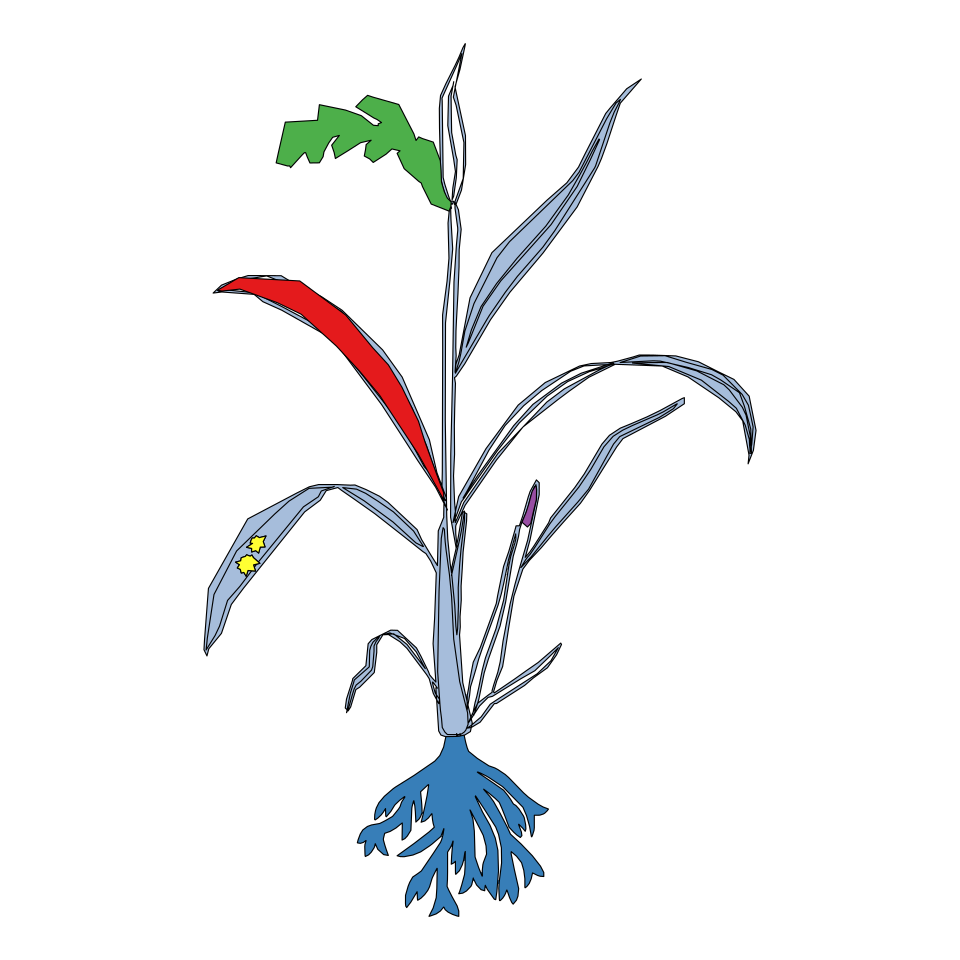

Plant anatogram in ggplot2

Oryza sativa

# install.packages("remotes")
# remotes::install_github("jespermaag/gganatogram")
library(gganatogram)

gganatogram(data = other_key$oryza_sativa.whole_plant,
            organism = "oryza_sativa.whole_plant",
            fillOutline = "#a6bddb", fill = "colour") +
  theme_void() +
  coord_fixed()