Sample data
For this tutorial we are going to use a subset of the diamonds data set from ggplot2 package.
# install.packages("ggplot2")
library(ggplot2)

# Sample data
df <- diamonds[1:100, c("color", "depth")]
Ridgeline plots (joy plots) with geom_density_ridges
The geom_density_ridges function from the ggridges package allows creating a ridgeline visualization. Given a numerical variable (depth) and a categorical variable (color) a density estimation of the data will be calculated and displayed for each group.
# install.packages("ggridges")
library(ggridges)
# install.packages("ggplot2")
library(ggplot2)

ggplot(df, aes(x = depth, y = color)) +
  geom_density_ridges()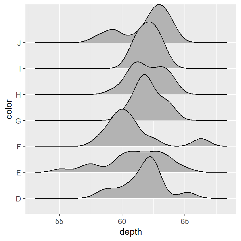
geom_density_ridges2
Note that there is an equivalent function named geom_density_ridges2 which uses closed polygons to display the density estimates, so the line will also appear at the bottom of each density estimation.
# install.packages("ggridges")
library(ggridges)
# install.packages("ggplot2")
library(ggplot2)

ggplot(df, aes(x = depth, y = color)) +
  geom_density_ridges2()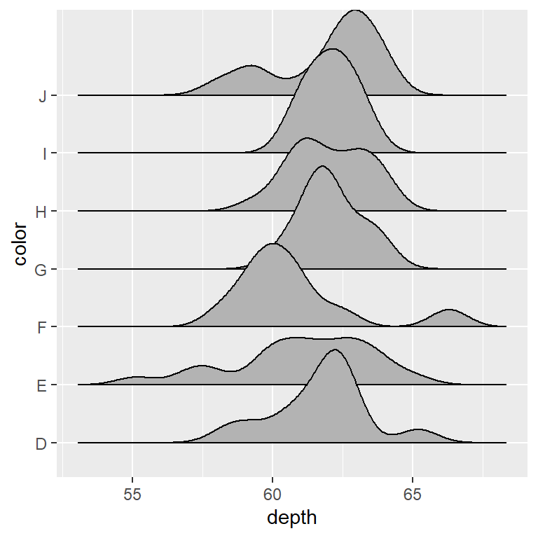
Cut the trailing tails
The rel_min_height argument of the function can be used to cut the trailing tails. You will need to fine tune the value depending on your data.
# install.packages("ggridges")
library(ggridges)
# install.packages("ggplot2")
library(ggplot2)

ggplot(df, aes(x = depth, y = color)) +
  geom_density_ridges(rel_min_height = 0.005)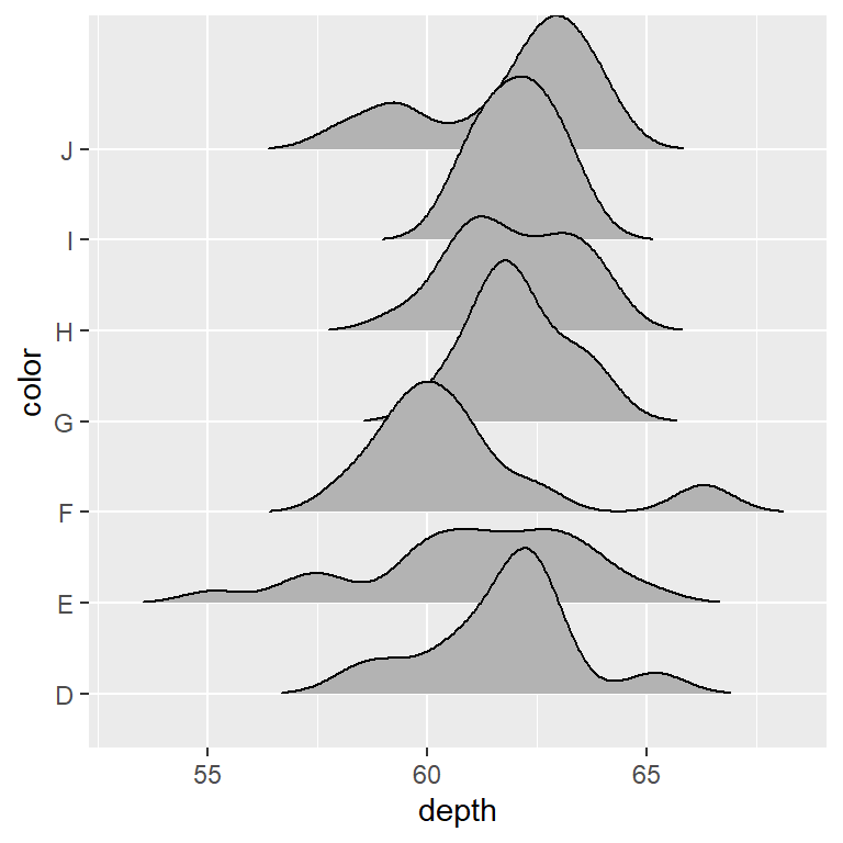
Scale
In addition, the scale argument controls the scaling of the ridgelines relative to the spacing between them.
# install.packages("ggridges")
library(ggridges)
# install.packages("ggplot2")
library(ggplot2)

ggplot(df, aes(x = depth, y = color)) +
  geom_density_ridges(scale = 3)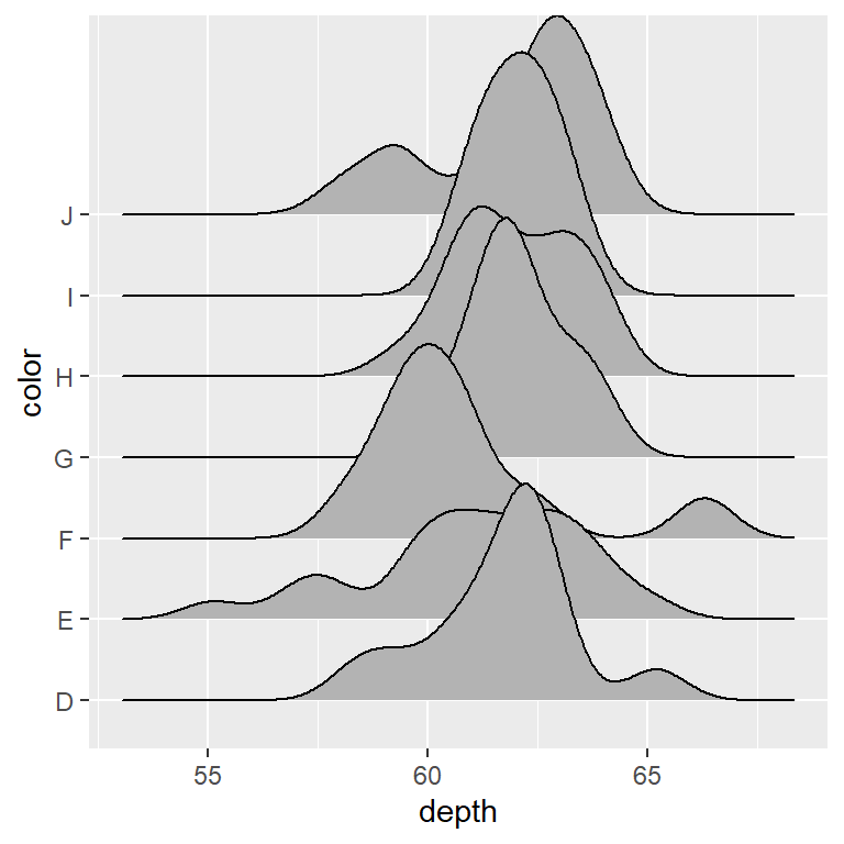
Alternative stats
The stat argument can be used to select the statistical transformation to be used.
# install.packages("ggridges")
library(ggridges)
# install.packages("ggplot2")
library(ggplot2)

ggplot(df, aes(x = depth, y = color)) +
  geom_density_ridges(stat = "binline",
                      bins = 20, draw_baseline = FALSE)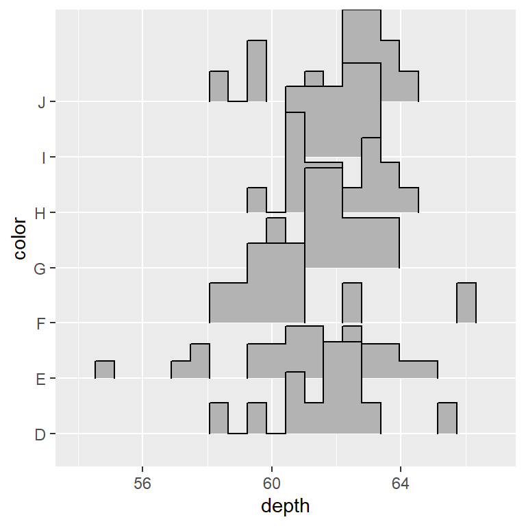
Color customization
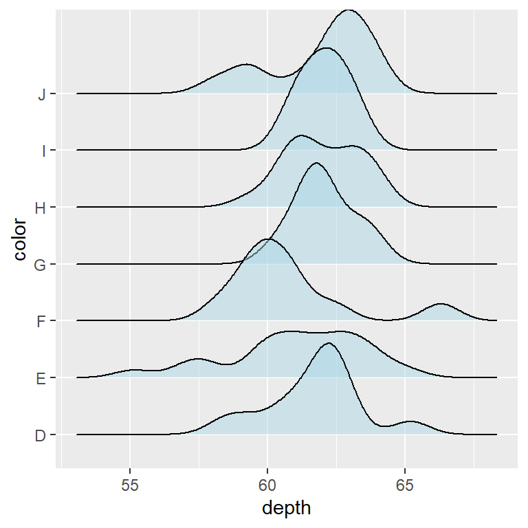
Fill color and transparency
The default gray color of the ridgelines can be changed with the fill argument of the geom_density_ridges function. Note that you can also specify a level of transparency with alpha.
# install.packages("ggridges")
library(ggridges)
# install.packages("ggplot2")
library(ggplot2)

ggplot(df, aes(x = depth, y = color)) +
  geom_density_ridges(fill = "lightblue", alpha = 0.5)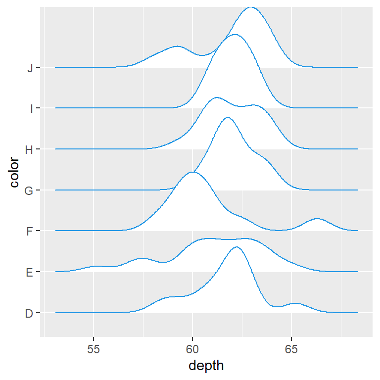
Border color
The color argument of the function controls the color of the lines. As in other plots you can also change the line type and the width of the lines.
# install.packages("ggridges")
library(ggridges)
# install.packages("ggplot2")
library(ggplot2)

ggplot(df, aes(x = depth, y = color)) +
  geom_density_ridges(fill = "white",
                      color = 4,
                      linetype = 1,
                      lwd = 0.5)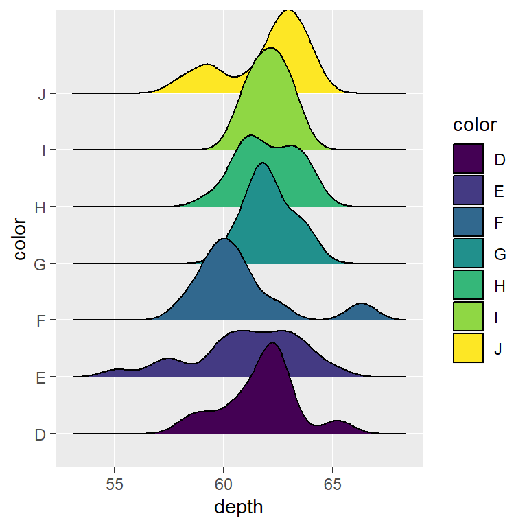
Color based on group
You can also fill the densities based on the categorical variable, passing it to the fill argument of aes. The color palette can be changed with scale_fill_manual, for instance.
# install.packages("ggridges")
library(ggridges)
# install.packages("ggplot2")
library(ggplot2)

ggplot(df, aes(x = depth, y = color, fill = color)) +
  geom_density_ridges()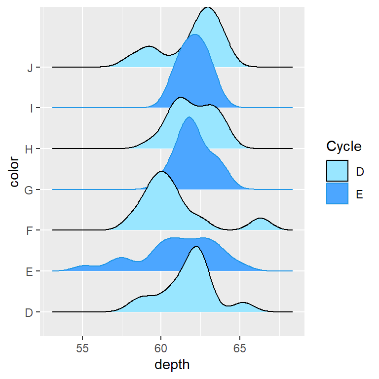
Cyclical color scales
The scale_fill_cyclical and scale_color_cyclical functions can be used to add cyclical fill and border colors to the density estimations.
# install.packages("ggridges")
library(ggridges)
# install.packages("ggplot2")
library(ggplot2)

ggplot(df, aes(x = depth, y = color, fill = color, color = color)) +
  geom_density_ridges() +
  scale_fill_cyclical(name = "Cycle", guide = "legend",
                      values = c("#99E6FF", "#4CA6FF")) +
  scale_color_cyclical(name = "Cycle", guide = "legend",
                       values = c(1, 4))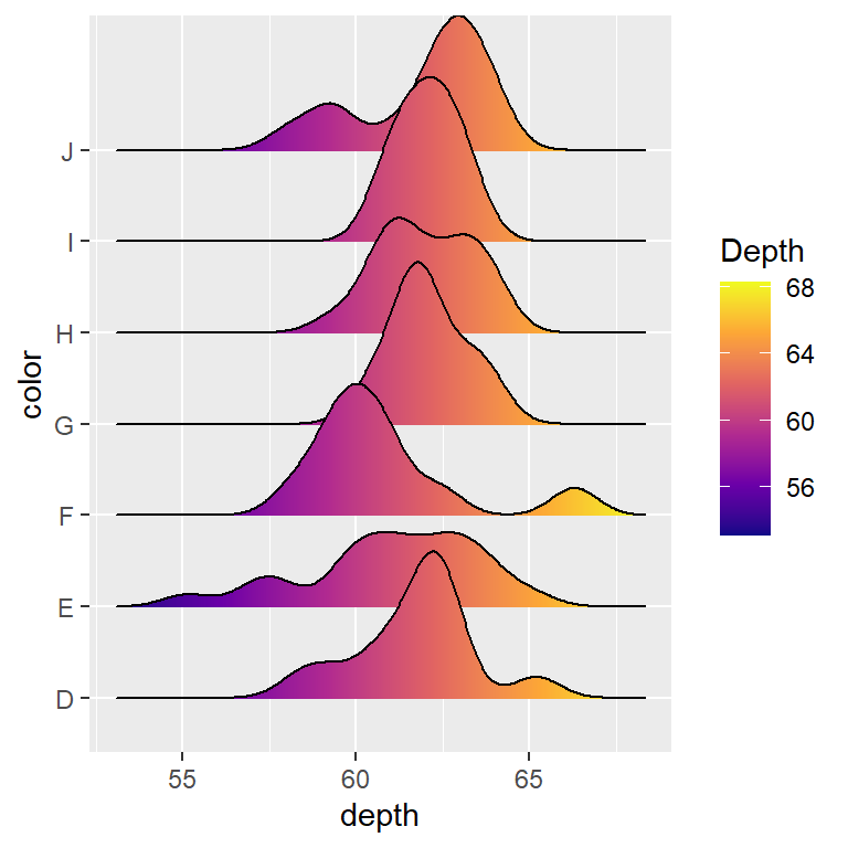
Gradient
You can pass stat(x) or factor(stat(x)) to the fill argument of aes and use geom_density_ridges_gradient and a continuous fill color scale to fill each ridgeline with a gradient.
# install.packages("ggridges")
library(ggridges)
# install.packages("ggplot2")
library(ggplot2)

ggplot(df, aes(x = depth, y = color, fill = stat(x))) +
  geom_density_ridges_gradient() +
  scale_fill_viridis_c(name = "Depth", option = "C")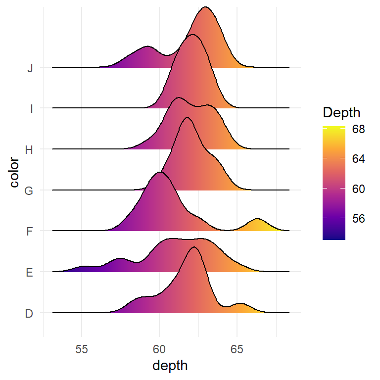
Change the theme
Note that you can also change the ggplot2 theme to modify the appearance of the plot. The ggridges package provides the theme_ridges theme.
# install.packages("ggridges")
library(ggridges)
# install.packages("ggplot2")
library(ggplot2)

ggplot(df, aes(x = depth, y = color, fill = stat(x))) +
  geom_density_ridges_gradient() +
  scale_fill_viridis_c(name = "Depth", option = "C") +
  coord_cartesian(clip = "off") + # To avoid cut off
  theme_minimal()
Adding quantiles and probabilities with stat_density_ridges
If you use stat_density_ridges instead of geom_density_ridges and set the quantile_lines argument to TRUE the quantiles will be calculated and displayed for each density.
# install.packages("ggridges")
library(ggridges)
# install.packages("ggplot2")
library(ggplot2)

ggplot(df, aes(x = depth, y = color)) +
  stat_density_ridges(quantile_lines = TRUE, alpha = 0.75)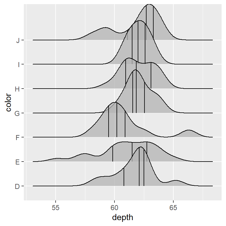
Number of quantiles
The quantiles argument controls which or how how many quantiles are displayed. If you pass an integer the data will be cut into that many equal quantiles.
# install.packages("ggridges")
library(ggridges)
# install.packages("ggplot2")
library(ggplot2)

ggplot(df, aes(x = depth, y = color)) +
  stat_density_ridges(quantile_lines = TRUE, alpha = 0.75,
                      quantiles = 2)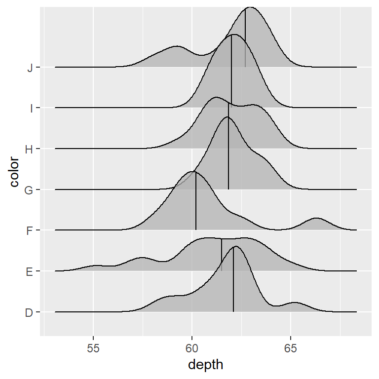
Specify the quantiles
If you pass a value or a vector of values between 0 and 1 to the quantiles argument those quantiles will be calculated and displayed.
# install.packages("ggridges")
library(ggridges)
# install.packages("ggplot2")
library(ggplot2)

ggplot(df, aes(x = depth, y = color)) +
  stat_density_ridges(quantile_lines = TRUE, alpha = 0.75,
                      quantiles = c(0.05, 0.5, 0.95))
Color by quantile
Passing stat(quantile) to fill and setting calc_ecdf and geom = "density_ridges_gradient" each quantiles will be filled with a different color. Note that if you set quantile_lines = TRUE the vertical lines for each quantile will be drawn.
# install.packages("ggridges")
library(ggridges)
# install.packages("ggplot2")
library(ggplot2)

ggplot(df, aes(x = depth, y = color, fill = stat(quantile))) +
  stat_density_ridges(quantile_lines = FALSE,
                      calc_ecdf = TRUE,
                      geom = "density_ridges_gradient") +
  scale_fill_brewer(name = "")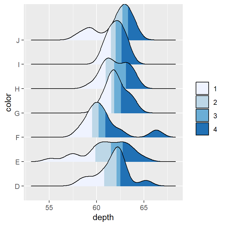
Highlight the tails of the distribution
The same approach described above can be used to highlight the tails of the distributions.
# install.packages("ggridges")
library(ggridges)
# install.packages("ggplot2")
library(ggplot2)

ggplot(df, aes(x = depth, y = color, fill = stat(quantile))) +
  stat_density_ridges(quantile_lines = TRUE,
                      calc_ecdf = TRUE,
                      geom = "density_ridges_gradient",
                      quantiles = c(0.05, 0.95)) +
  scale_fill_manual(name = "Prob.", values = c("#E2FFF2", "white", "#B0E0E6"),
                    labels = c("(0, 5%]", "(5%, 95%]", "(95%, 1]"))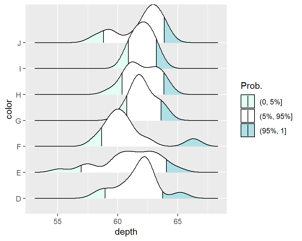
Mapping the tails probabilities onto color
Similarly, using stat(ecdf) it is possible to add a gradient to the densities displaying the tail probabilities.
# install.packages("ggridges")
library(ggridges)
# install.packages("ggplot2")
library(ggplot2)

ggplot(df, aes(depth, y = color,
               fill = 0.5 - abs(0.5 - stat(ecdf)))) +
  stat_density_ridges(geom = "density_ridges_gradient", calc_ecdf = TRUE) +
  scale_fill_gradient(low = "white", high = "#87CEFF",
                      name = "Tail prob.")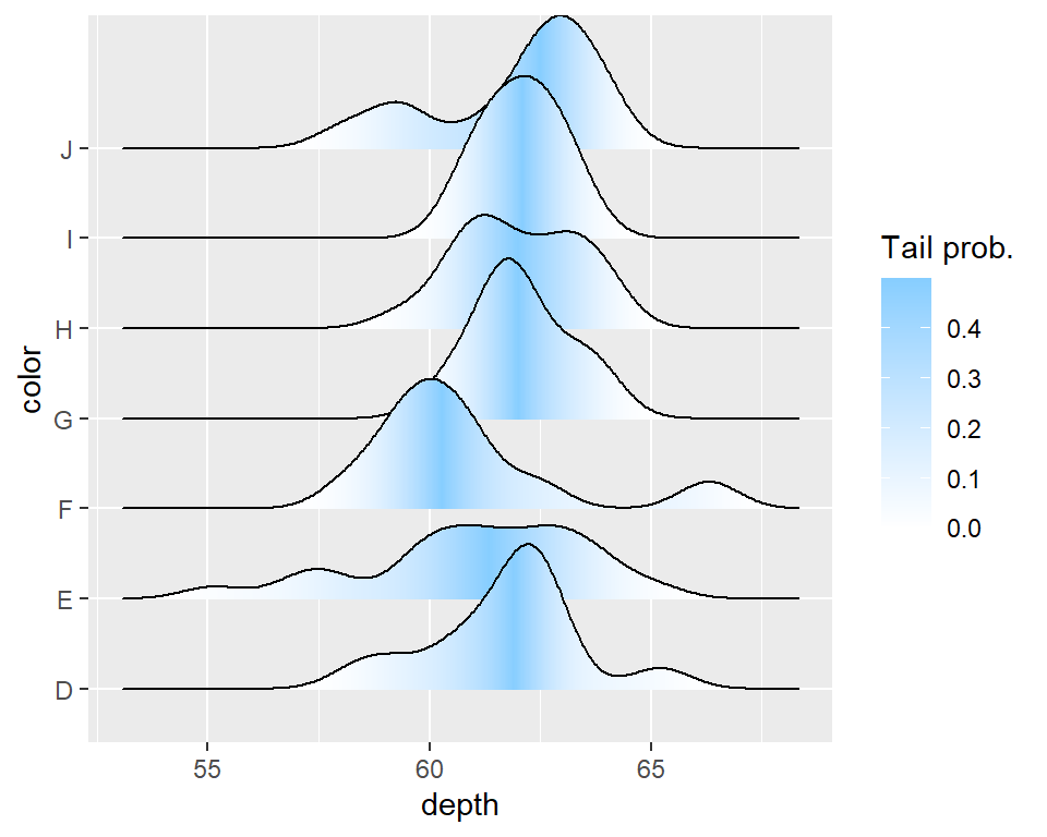

Master Statistics
Learn statistics from the basics to advanced techniques, clearly explained
Go to site