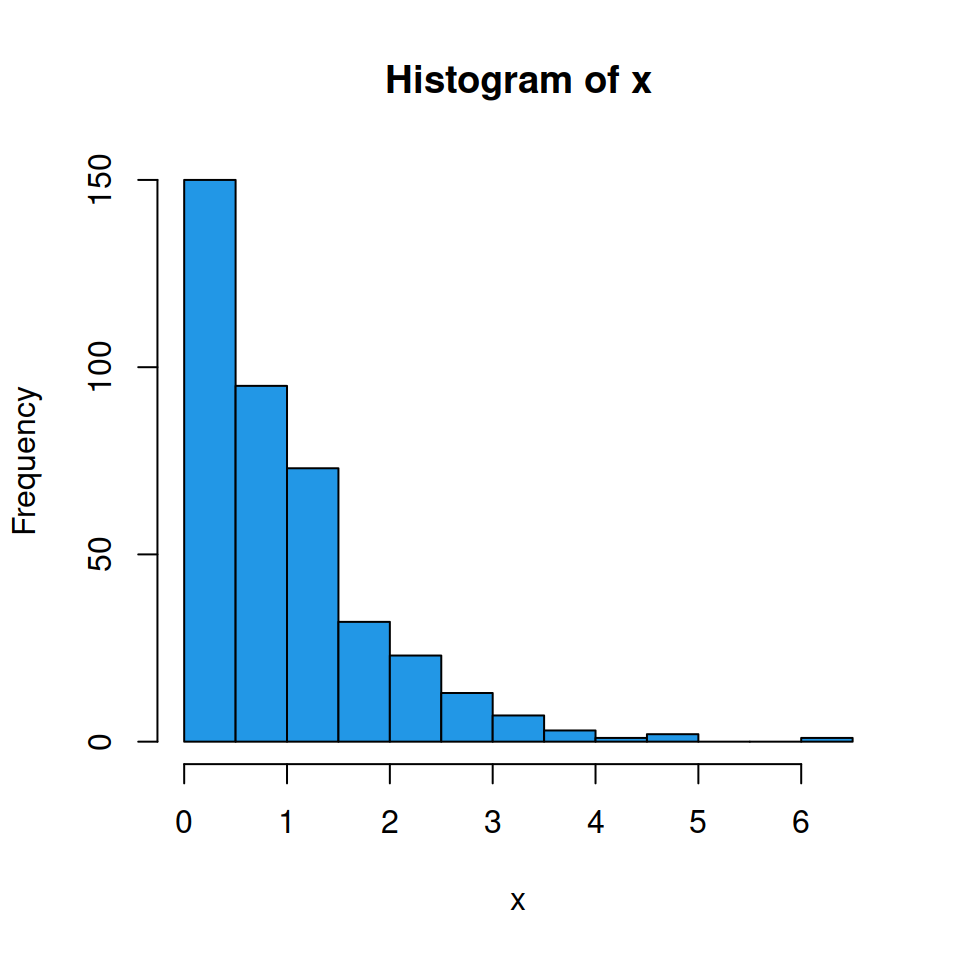
A basic density histogram
The hist function creates frequency histograms by default. You can override this behaviour by setting prob = TRUE or freq = FALSE.
# Sample data (normal)
set.seed(1)
x <- rnorm(400)

# Histogram
hist(x, prob = TRUE)
hist(x, freq = FALSE) # Equivalent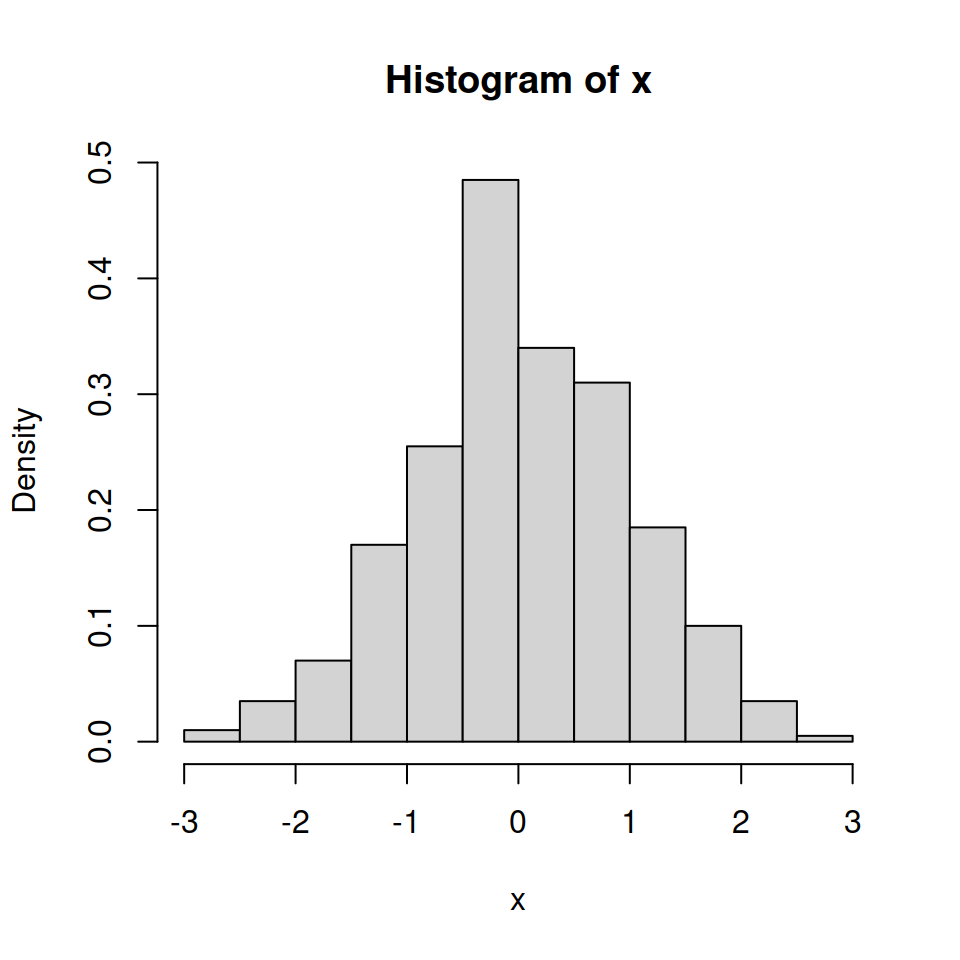
Color of the histogram
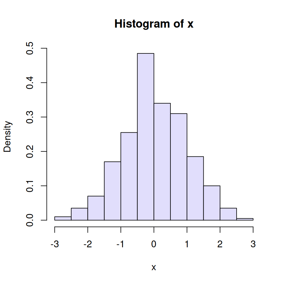
You can change the default fill color of the histogram bars (gray since R 4.0.0) to other making use of the col argument.
# Sample data (normal)
set.seed(1)
x <- rnorm(400)

# Blue histogram
hist(x,
     prob = TRUE,
     col = "#E1DEFC") # Color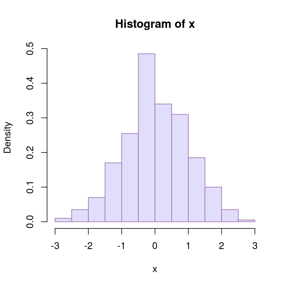
The border argument allows modifying the border color of the bars.
# Sample data (normal)
set.seed(1)
x <- rnorm(400)

# Purple histogram
hist(x,
     prob = TRUE,
     col = "#E1DEFC",    # Fill color
     border = "#9A68A4") # Border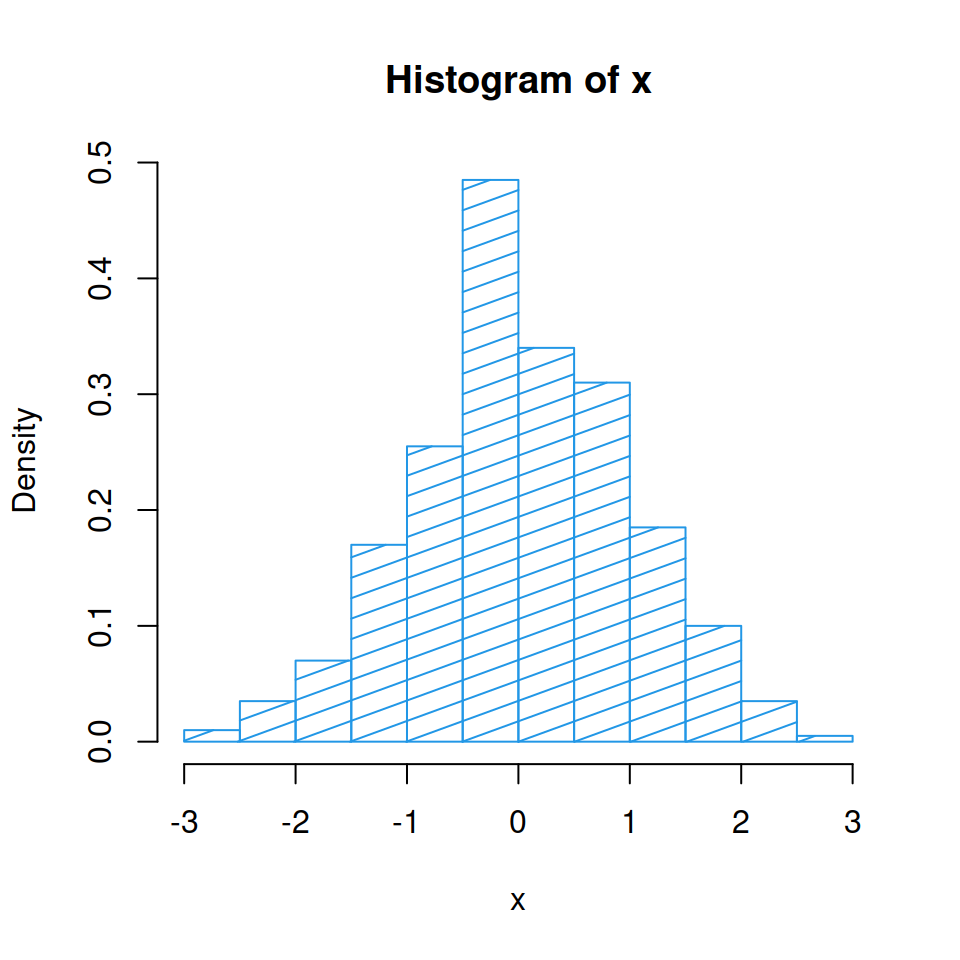
You can also use shading lines instead of a fill color. Set them with the density argument and modify its angle with angle.
# Sample data (normal)
set.seed(1)
x <- rnorm(400)

# White histogram with shading lines
hist(x,
     prob = TRUE,
     col = 4,      # Color
     density = 10, # Shading lines
     angle = 20)   # Shading lines angle
Titles and labels
You can also modify the title, subtitle, and axes labels with main, sub, xlab and ylab arguments, respectively.
# Sample data (normal)
set.seed(1)
x <- rnorm(400)

# Histogram with titles
hist(x,
     prob = TRUE,
     main = "Title of the histogram", # Title
     sub = "Subtitle",                # Subtitle
     xlab = "X-axis label",           # X-axis label
     ylab = "Y-axis label")           # Y-axis label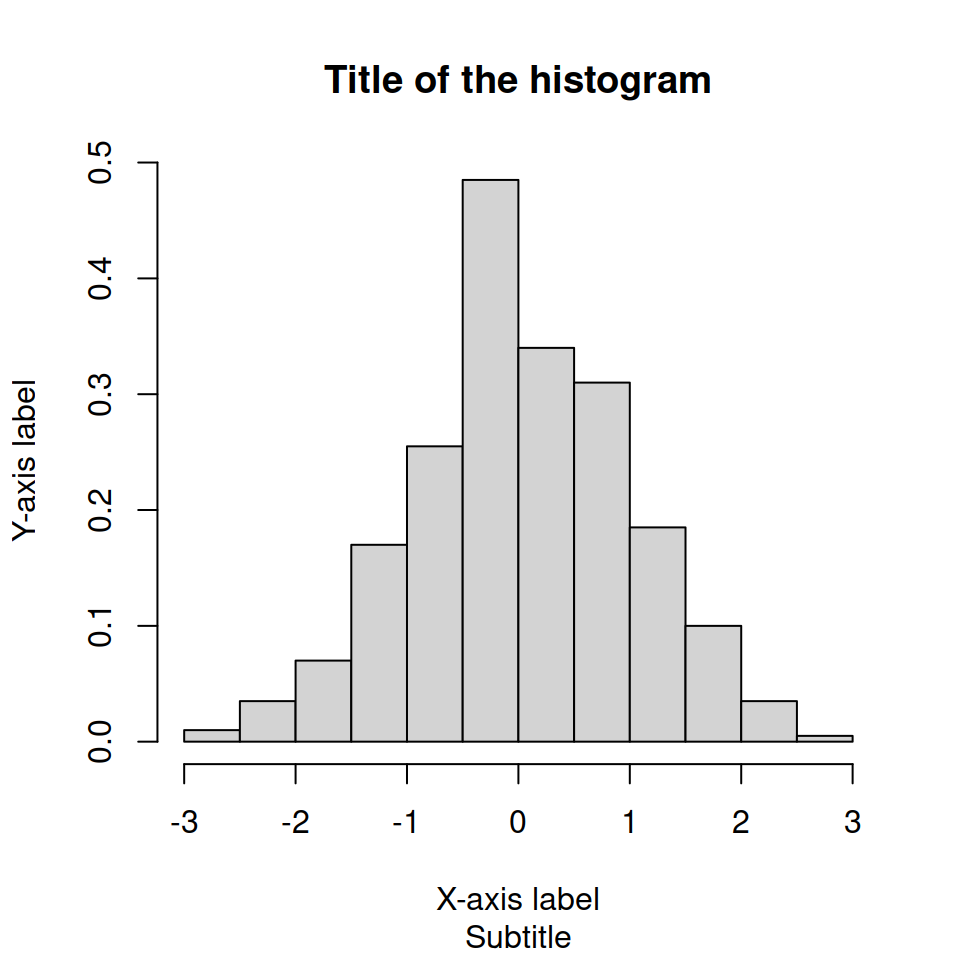

Master Statistics
Learn statistics from the basics to advanced techniques, clearly explained
Go to site