Dynamic maps with leaflet
The leaflet package allows creating dynamic and interactive maps using the Leaflet JavaScript library. The main advantage of using leaflet is its flexibility and that using leaflet in R is really easy.
In order to create a simple map you will need to load the package and then use the leaflet function and then add new layers with the pipe operator (%>%). With addTiles you will add the default base map and with setView you will be able to set a center point and a zoom level.
library(leaflet)

leaflet() %>%
  addTiles() %>%
  setView(lng = -3.7, lat = 40.4, zoom = 5)
Markers
It is possible to add different types of markers to the maps. The most common functions are addMarkers, which will add icon markers (and accepts custom markers) and addCircleMarkers, which will add circular markers that can be customized.
You can add a single marker to the plot by passing coordinates to the lng (longitude) and lat (latitude) arguments of the addMarkers function. The function allows a single value or a vector of values as input for each argument.
library(leaflet)

leaflet() %>%
  addTiles() %>%
  setView(lng = -3.7, lat = 40.4, zoom = 5) %>%
  addMarkers(lng = -3.7, lat = 40.4)
Multiple markers from a data frame
Note that there are several ways to input data. For instance, if your data comes from a data frame you can input the data frame to data. Recall that the column names must be lng and lat.
library(leaflet)

leaflet() %>%
  addTiles() %>%
  setView(lng = -3.7, lat = 40.4, zoom = 5) %>%
  addMarkers(data = data.frame(lng = c(-3.7, -8, -4.2), lat = c(40.4, 43.1, 41.4)))
Markers with custom icons
A very useful argument of the addMarkers function is icon, which allows a list as input to set custom markers. The list can be created easily with icons, a function that requires, at least the specification of an iconUrl with the image or images, the iconWidth and the iconHeight to set the size for all or each icon.
library(leaflet)

# Data
df <- data.frame(lng = c(12.5, 14.3, 11.234),
                 lat = c(42, 41, 43.84),
                 group = c("A", "B", "A"))

# Icons
icons_list <- icons(iconUrl = ifelse(df$group == "A",
                     'https://raw.githubusercontent.com/R-CoderDotCom/samples/main/marker.png',
                     ifelse(df$group == "B", "https://raw.githubusercontent.com/R-CoderDotCom/chinchet/main/inst/red.png", NA)),
                     iconWidth = c(50, 90, 40), iconHeight = c(50, 90, 40))

leaflet() %>%
  addTiles() %>%
  setView(lng = 12.43, lat = 42.98, zoom = 6) %>%
  addMarkers(data = df, icon = icons_list)
Circle markers
Circle markers can be drawn with addCircleMarkers. These markers can be added the same way as the previous markers, but the main difference is that you can customize its color with color. You can also set the radius of the markers with radius, measured in pixels.
library(leaflet)

circles <- data.frame(lng = c(23.59, 34.95, 17.47),
                      lat = c(-3.53, -6.32, -12.24))

leaflet() %>%
  addTiles() %>%
  addCircleMarkers(data = circles, color = "red")
Polygons and polylines
You can overlay polygons or spatial polygons to the maps from a shapefile or geojson. You will need to import your data with sf, rgdal or a similar package. We will use sf in our examples. In order to add the polygons you will need to input the data to the addPolygons function.
library(leaflet)
library(sf)

# Read a Geojson or shapefile
data_map <- read_sf("https://raw.githubusercontent.com/R-CoderDotCom/data/main/sample_geojson.geojson")

# Transform to leaflet projection if needed
data_map <- st_transform(data_map, crs = '+proj=longlat +datum=WGS84')

leaflet() %>%
  addTiles() %>%
  setView(lng = -0.49, lat = 38.34, zoom = 14) %>%
  addPolygons(data = data_map, color = "blue", stroke = 1, opacity = 0.8)
Note that depending on your data you will also need to transform it to the leaflet projection (+proj=longlat +datum=WGS84).
Circles
Circles can be added with the addCircles function. These circles are very similar to circle markers but the radius argument sets the radius in meters instead of pixels and can be used for instance, for creating influence areas.
library(leaflet)

circles <- data.frame(lng = c(-3.7, -3.72),
                      lat = c(40.4, 40.42))

leaflet() %>%
  addTiles() %>%
  setView(lng = -3.7, lat = 40.4, zoom = 13) %>%
  addCircleMarkers(data = circles, color = "red") %>%
  addCircles(data = circles, radius = 2000)
Rectangles
Instead of circles you can add rectangles with addRectangles but you will need to input the coordinates for the south-west (lng1 and lat1) and north-east (lng2 and lat2) corners of the rectangle to be drawn.
library(leaflet)

leaflet() %>%
  addTiles() %>%
  setView(lng = -77.04, lat = -12.05, zoom = 11) %>%
  addRectangles(lng1 = -77.08, lat1 = -12.1,
                lng2 = -76.95, lat2 = -11.98)
Colors
The colors of the circles, rectangles, polygons and other elements can be customized with color and its transparency with opacity. Some elements such as circles include the fillColor and fillOpacity arguments that will change the fill color while the other arguments would be used to customize the border color, as in the example below.
library(leaflet)

circles <- data.frame(lng = c(-3.7, -3.72),
                      lat = c(40.4, 40.42))

leaflet() %>%
  addTiles() %>%
  setView(lng = -3.7, lat = 40.4, zoom = 13) %>%
  addCircles(data = circles, radius = 2000,
             color = "blue",  opacity = 1,
             fillColor = "red", fillOpacity = 0.25)
You can also pass a vector of colors as input based on some conditions, e.g. ifelse(data$var > 1, "red", "blue") would assign red for values greater than 1 and blue for the rest.
Continuous color palette
You can also assign the elements to a continuous color palette. For this purpose you can use a function for color mapping, such as colorNumeric and then you will need to apply the palette to color. In the following example we are creating a choropleth map in Leaflet.
library(leaflet)
library(sf)

# Read a Geojson or shapefile
data_map <- read_sf("https://raw.githubusercontent.com/R-CoderDotCom/data/main/sample_geojson.geojson")

# Transform to leaflet projection if needed
data_map <- st_transform(data_map, crs = '+proj=longlat +datum=WGS84')

# Continuous palette
pal <- colorNumeric(palette = "viridis", domain = data_map$tot_pob)

leaflet() %>%
  addTiles() %>%
  setView(lng = -0.49, lat = 38.34, zoom = 14) %>%
  addPolygons(data = data_map, color = pal(data_map$tot_pob), stroke = 1, opacity = 0.8)
Discrete color palette
If your data is categorized you can also set colors based on that categorical variable. In this scenario you can use a color function such as colorFactor to map the groups to colors.
library(leaflet)
library(sf)

# Read a Geojson or shapefile
data_map <- read_sf("https://raw.githubusercontent.com/R-CoderDotCom/data/main/sample_geojson.geojson")

# Transform to leaflet projection if needed
data_map <- st_transform(data_map, crs = '+proj=longlat +datum=WGS84')

# Discrete palette
data_map$tot_pob_cat <- cut(data_map$tot_pob, breaks = 3)
pal <- colorFactor("plasma", levels = levels(data_map$tot_pob_cat))

leaflet() %>%
  addTiles() %>%
  setView(lng = -0.49, lat = 38.34, zoom = 14) %>%
  addPolygons(data = data_map, color = pal(data_map$tot_pob_cat), stroke = 1, opacity = 0.8)
Pop ups
Pop ups can appear when you click over a marker, a polygon, a rectangle, etc. making use of the popup argument. These popups can be used to display important information about a point or a region, such as its population. The argument takes a string as input and admits HTML and inline CSS styles.
library(leaflet)

circles <- data.frame(lng = c(-73.58, -73.46), lat = c(45.5, 45.55))

leaflet() %>%
  addTiles() %>%
  setView(lng = -73.53, lat = 45.5, zoom = 12) %>%
  addCircles(data = circles, radius = 2000,
             popup = paste0("Title", "<hr>", "Text 1", "<br>", "Text 2")) %>%
  addCircleMarkers(data = circles,
                   popup = c("A", "B"))
You might need to order your layers when using popups. For instance, if you add points and then circles over them, you won’t be able to click over the markers, so you will need to add the circles and then the markers and then both elements will be clickable.
Basemaps
The default map style added with addTiles can be changed with addProviderTiles. After importing leaflet you will have access to a list named providers which elements can be passed as input to the addProviderTiles function, as in the examples below. Check this list to preview different themes.
“CartoDB.Positron”
In this example we are setting the CartoDB.Positron base map, which is widely used.
library(leaflet)

leaflet() %>%
  addProviderTiles(providers$CartoDB.Positron) %>%
  setView(lng = 13.4, lat = 52.52, zoom = 14)
“Esri.WorldImagery”
In this example we are setting the Esri.WorldImagery map style, which allows to visualize the map with real images.
library(leaflet)

leaflet() %>%
  addProviderTiles(providers$Esri.WorldImagery) %>%
  setView(lng = 13.4, lat = 52.52, zoom = 14)
Legend
With addLegend you can add a legend to Leaflet maps. You will need to input the values and the color palette in addition to the position or the title, as shown in the following block of code.
library(leaflet)

circles <- data.frame(lng = c(-3.7, -8, -4.2),
                      lat = c(40.4, 43.1, 41.4),
                      values = c(10, 20, 30))

# Continuous palette
# pal <- colorNumeric(palette = "viridis", domain = circles$values)

# Discrete palette
pal <- colorFactor("viridis", levels = circles$values)

leaflet() %>%
  addTiles() %>%
  setView(lng = -3.7, lat = 40.4, zoom = 5) %>%
  addCircleMarkers(data = circles, color = ~pal(values)) %>%
  addLegend(data = circles,
            position = "bottomright",
            pal = pal, values = ~values,
            title = "Legend",
            opacity = 1)
👉 Tip: use ~ to avoid specifying the data set name if you already passed it to data.
Other features
Select and unselect layers
With addLayersControl you will be able to select and unselect different layers of the plot. You will need to assign each layer a name with group and then use the function to set the baseGroups (layers that can be selected only one at time) and the overlayGroups (layers that can be selected independently).
library(leaflet)

leaflet() %>%
  addTiles(group = "StreetMap") %>%
  addProviderTiles(providers$Stamen.Watercolor, group = "Stamen") %>%
  addMarkers(lng = c(-102.8, -101.1), lat = c(38.7, 39.4), group = "Markers") %>%
  addLayersControl(baseGroups = c("StreetMap", "Stamen"), overlayGroups = c("Markers"),
                   position = "topright")
Add measurement
You can add a measurement tool with the addMeasure function. This function provides several arguments to customize its position, metrics and colors. Once added, you will need to click over the tool and start adding measures.
library(leaflet)

leaflet() %>%
  addTiles() %>%
  setView(lng = -101.6, lat = 39.86, zoom = 3) %>%
  addMeasure(
    position = "bottomleft",
    primaryLengthUnit = "meters",
    primaryAreaUnit = "sqmeters",
    activeColor = "#3D535D",
    completedColor = "#7D4479")
Add graticule
A graticule is a grid added on top of the map dividing it in different sections. You can add a graticule with addSimpleGraticule function or with addGraticule function, which allows to customize the style of the grid passing a list to style, e.g. addGraticule(style = list(color = "#333", weight = 1)).
library(leaflet)

leaflet() %>%
  addTiles() %>%
  setView(lng = -3.7, lat = 40.4, zoom = 2) %>%
  addSimpleGraticule()
Add a daylight layer
The addTerminator function adds a daylight layer on top of the map. By default the layer is based on the execution time, but you can customize it with the time argument.
library(leaflet)

leaflet() %>%
  addTiles() %>%
  addTerminator()
Add a minimap
With the addMiniMap function you can add a mini map over the plot, so you will be able to see where you are despite the level of zoom. This function provides several arguments to customize the size, colors (aimingRectOptions), the shadow (shadowRectOptions) and other features.
library(leaflet)

leaflet() %>%
  addTiles() %>%
  setView(lng = 2.4, lat = 46.6, zoom = 5) %>%
  addMiniMap(width = 150, height = 150)
Additional plugins with leaflet.extras
leaflet.extras is an incredible useful library to use with leaflet, as it provides lots of additional plugins that are not available in the core package. Some of the functions of leaflet.extras are highlighted in this section, but recall to read the original documentation for further functions and details.
Add a drawing toolbar
Drawing over Leaflet can be very useful for Shiny applications or to illustrate something in real time. You will also be able to retrieve the coordinates of the draws.
library(leaflet)
library(leaflet.extras)

leaflet() %>%
  addTiles() %>%
  setView(lng = -73, lat = 3.5, zoom = 5) %>%
  addDrawToolbar()
Add a measurement tool
Other interesting tool is the measurement tool, which will allow you to measure the displayed areas.
library(leaflet)
library(sf)
library(leaflet.extras)

data_map <- read_sf("https://raw.githubusercontent.com/R-CoderDotCom/data/main/sample_geojson.geojson")
data_map <- st_transform(data_map, crs = '+proj=longlat +datum=WGS84')

leaflet() %>%
  addTiles() %>%
  enableMeasurePath() %>%
  setView(lng = -0.49, lat = 38.34, zoom = 14) %>%
  addPolygons(data = data_map, color = "blue", stroke = 1, opacity = 0.8) %>%
  addMeasurePathToolbar(options = measurePathOptions(imperial = FALSE,
                                                     minPixelDistance = 100,
                                                     showDistances = FALSE,
                                                     showOnHover = TRUE))
Master Statistics
Learn statistics from the basics to advanced techniques, clearly explained
Go to site