Mapping in ggplot2 with maps, geom_polygon and geom_map
Data from a package
There are several ways to plot a map in R with ggplot2 depending on the input data. The easiest way is to import a map from a package, such as the maps or rnaturalearth packages, but in this tutorial we are going to use maps. In order to use one of the maps from that package in ggplot2 you will need to use the map_data function from ggplot2, which will convert the map into a suitable data frame.
In the following example we are loading the world map. In order to plot the map you can use the geom_polygon or the geom_map functions as displayed below.
# install.packages("ggplot2")
# install.packages("maps")
library(ggplot2)
library(maps)
# Import the data with coordinates
world <- map_data("world")
# Plot the map. group = group connects the points in the correct order
ggplot(data = world, aes(x = long, y = lat, group = group)) +
geom_polygon()
# Equivalent to:
ggplot(world, aes(map_id = region)) +
geom_map(data = world, map = world,
aes(x = long, y = lat, map_id = region))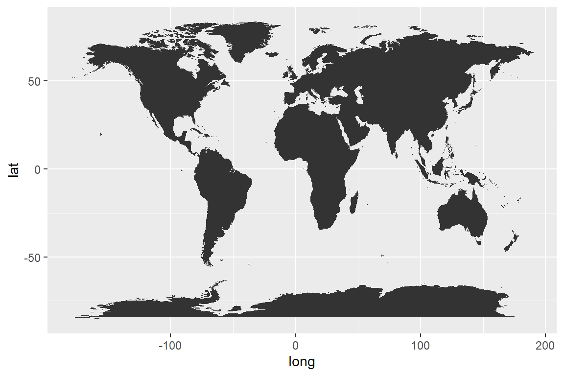
Plotting spatial data with sf and geom_sf
Data from a shapefile or geojson
Probably, the best way to create a map is to import a shapefile (.shp) or a geojson, but this means that you will need to make a research and look for the map you want to create. There are several resources to download maps in different formats, such as GISCO (see the giscoR package), opendatasoft or Efrain Maps, among others.
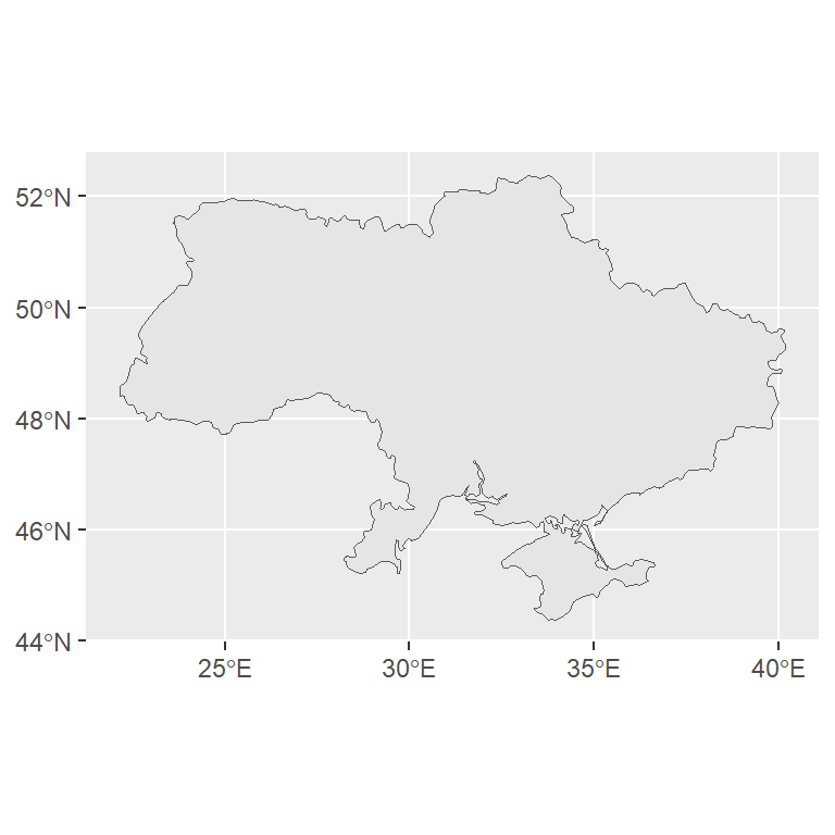
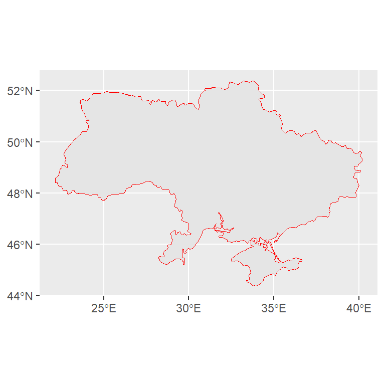
In order to read a geojson or shapefile you can make use of the read_sf function from sf. Then, you can pass the object to ggplot2 and use the geom_sf function that allows visualizing the simple features (sf) objects.
# install.packages("ggplot2")
# install.packages("sf")
library(ggplot2)
library(sf)
# Import a geojson or shapefile
map <- read_sf("https://raw.githubusercontent.com/R-CoderDotCom/data/main/ukraine.geojson")
ggplot(map) +
geom_sf()You can add more layers to the map, such as points or other geometries.
Coordinate systems
You can customize the coordinate system used to draw a map on ggplot2. If you want to check the coordinate reference system (CRS) of your geometry you can use the st_crs function from sf.
# install.packages("sf")
library(sf)
# Import a geojson or shapefile
map <- read_sf("https://raw.githubusercontent.com/R-CoderDotCom/data/main/ukraine.geojson")
# View the CRS
st_crs(map)
# Coordinate Reference System:
# User input: WGS 84
# wkt:
# GEOGCRS["WGS 84",
# DATUM["World Geodetic System 1984",
# ELLIPSOID["WGS 84",6378137,298.257223563,
# LENGTHUNIT["metre",1]]],
# PRIMEM["Greenwich",0,
# ANGLEUNIT["degree",0.0174532925199433]],
# CS[ellipsoidal,2],
# AXIS["geodetic latitude (Lat)",north,
# ORDER[1],
# ANGLEUNIT["degree",0.0174532925199433]],
# AXIS["geodetic longitude (Lon)",east,
# ORDER[2],
# ANGLEUNIT["degree",0.0174532925199433]],
# ID["EPSG",4326]]If you want to change the coordinate system you can use the coord_sf function. This function ensure that all layers use the same CRS and if none is specified it will use the CRS of the first geometry layer. You can also make use of the crs argument to specify a custom CRS, as in the example below:
# install.packages("ggplot2")
# install.packages("sf")
library(ggplot2)
library(sf)
# Import a geojson or shapefile
map <- read_sf("https://raw.githubusercontent.com/R-CoderDotCom/data/main/ukraine.geojson")
ggplot(map) +
geom_sf() +
coord_sf(crs = "+proj=robin")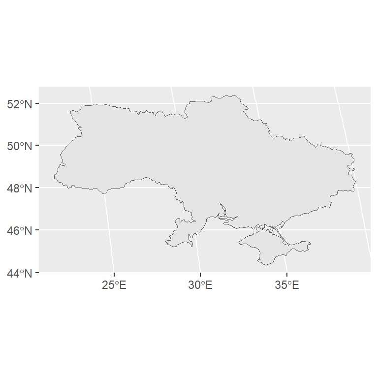
Recall that you could also use the st_transform function from sf to change the CRS of an sf object.
Colors
Fill color
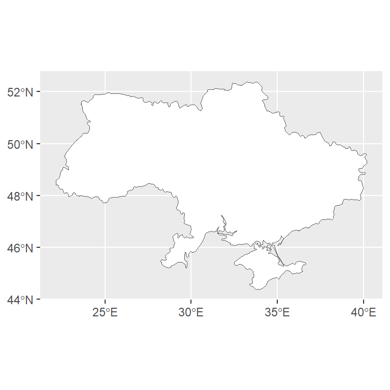
You can change the fill color of the map passing a color as input of the fill argument.
# install.packages("ggplot2")
# install.packages("sf")
library(ggplot2)
library(sf)
# Import a geojson or shapefile
map <- read_sf("https://raw.githubusercontent.com/R-CoderDotCom/data/main/ukraine.geojson")
ggplot(map) +
geom_sf(fill = "white")Border color
If you want to change the borders color of the geometries you can use the color argument.
# install.packages("ggplot2")
# install.packages("sf")
library(ggplot2)
library(sf)
# Import a geojson or shapefile
map <- read_sf("https://raw.githubusercontent.com/R-CoderDotCom/data/main/ukraine.geojson")
ggplot(map) +
geom_sf(color = "red")Color based on a numerical variable
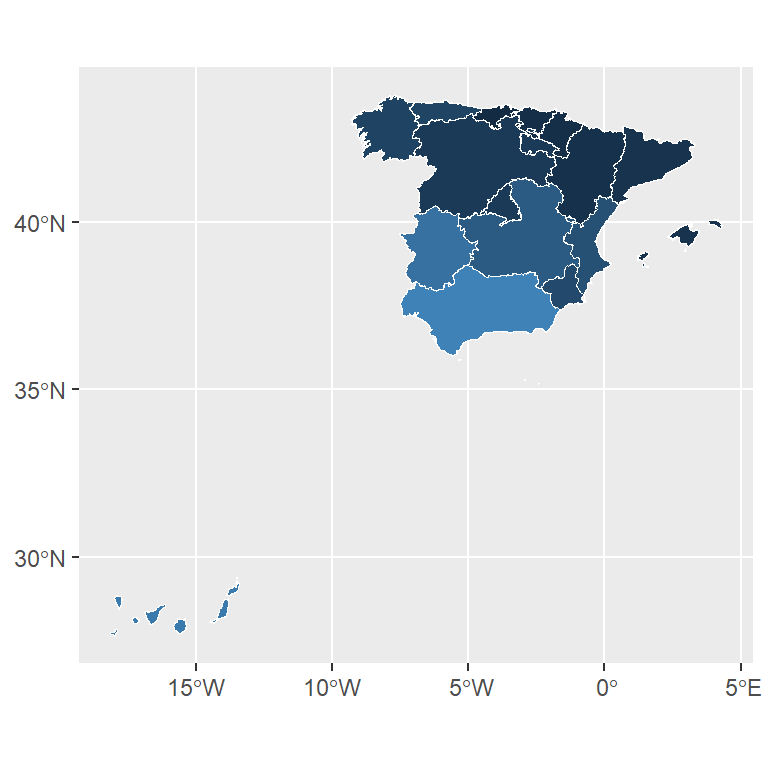
Note that you can also set the fill color based on a numerical variable representing some characteristic of each geographical area. For this purpose you will need to pass a numerical variable to the fill argument inside of aes. This kind of map is know as choropleth map.
# install.packages("ggplot2")
# install.packages("sf")
library(ggplot2)
library(sf)
# Import a geojson or shapefile
map <- read_sf("https://raw.githubusercontent.com/R-CoderDotCom/data/main/shapefile_spain/spain.geojson")
ggplot(map) +
geom_sf(color = "white", aes(fill = unemp_rate)) +
theme(legend.position = "none")Color based on a categorical variable
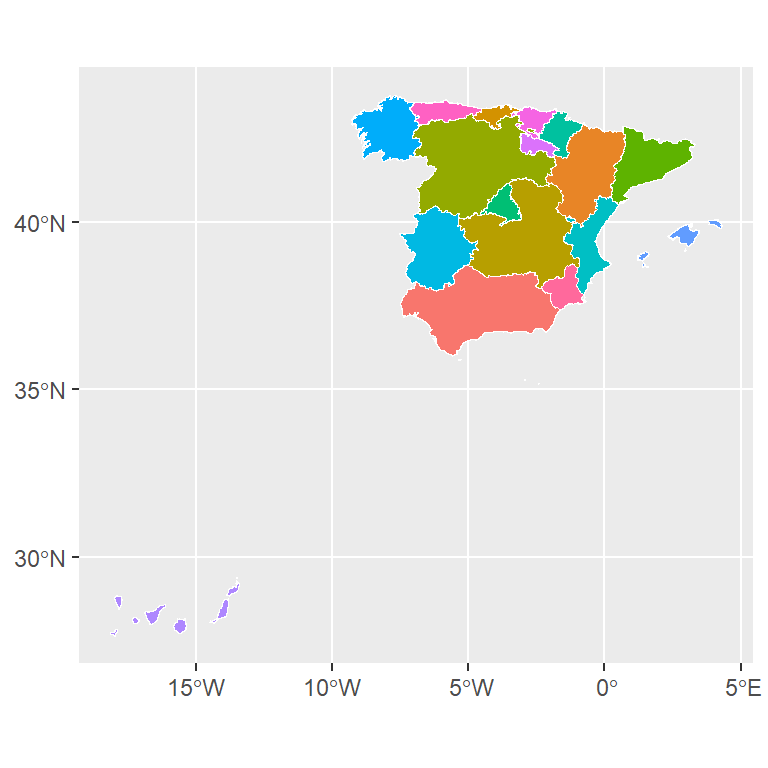
Instead of a numerical variable you can also pass a categorical variable representing groups. In the example below we are passing the names of each autonomous community of Spain, so each community will be displayed in a different color.
# install.packages("ggplot2")
# install.packages("sf")
library(ggplot2)
library(sf)
# Import a geojson or shapefile
map <- read_sf("https://raw.githubusercontent.com/R-CoderDotCom/data/main/shapefile_spain/spain.geojson")
ggplot(map) +
geom_sf(color = "white", aes(fill = name)) +
theme(legend.position = "none")Labels
It is possible to label the geometries of a map in ggplot2. There are several functions you can use, such as geom_text and geom_label or geom_sf_text and geom_sf_label if you are working with sf objects or even the geom_text_repel and geom_label_repel functions from ggrepel.
geom_sf_text and geom_sf_label
These functions can be used when you are working with an sf object. You will need to pass a variable with the texts to the label arguments inside aes. Note that you can also customize other styles of the texts, such as its size or color.
# install.packages("ggplot2")
# install.packages("sf")
library(ggplot2)
library(sf)
# Import a geojson or shapefile
map <- read_sf("https://raw.githubusercontent.com/R-CoderDotCom/data/main/shapefile_spain/spain.geojson")
ggplot(map) +
geom_sf(color = "white", aes(fill = unemp_rate)) +
geom_sf_text(aes(label = name), size = 2) +
theme(legend.position = "none")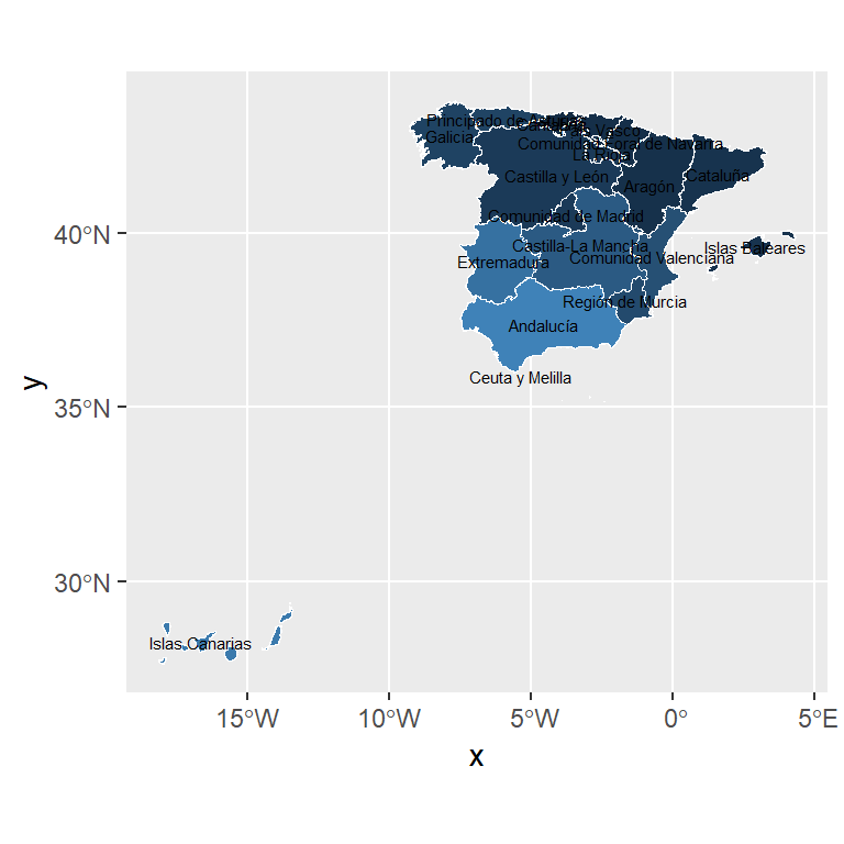
# install.packages("ggplot2")
# install.packages("sf")
library(ggplot2)
library(sf)
# Import a geojson or shapefile
map <- read_sf("https://raw.githubusercontent.com/R-CoderDotCom/data/main/shapefile_spain/spain.geojson")
ggplot(map) +
geom_sf(color = "white", aes(fill = unemp_rate)) +
geom_sf_label(aes(label = name), size = 2) +
theme(legend.position = "none")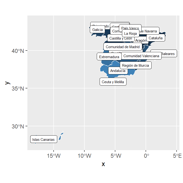
If your texts overlap, you can use the geom_text_repel or geom_label_repel functions from the ggrepel package, which will automatically try to fit the labels. If you are working with an sf object you will need to specify the geometry and the stat, as in the example below.
# install.packages("ggplot2")
# install.packages("sf")
# install.packages("ggrepel")
library(ggplot2)
library(sf)
# Import a geojson or shapefile
map <- read_sf("https://raw.githubusercontent.com/R-CoderDotCom/data/main/shapefile_spain/spain.geojson")
ggplot(map) +
geom_sf(color = "white", aes(fill = unemp_rate)) +
geom_text_repel(aes(label = name, geometry = geometry),
stat = "sf_coordinates", size = 3) +
theme(legend.position = "none")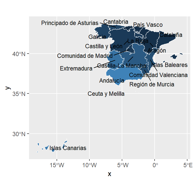
Interactive map
With the ggplotly function from plotly you can convert an static map made with ggplot2 into a interactive map. You just need to assign the map to an object and then apply the ggplotly function to that object.