Sample data
gt creates publication-quality tables with a grammar similar to ggplot2: start with data, pipe it to gt(), then add layers for formatting, styling and annotations. We will use the iris dataset throughout.
# install.packages("gt")
library(gt)

head(iris, 6)
gt()
Pipe any data frame into gt() to get a formatted HTML table immediately. Column names become headers and data types are detected automatically.
# install.packages("gt")
library(gt)

head(iris, 6) |>
gt()| Sepal.Length | Sepal.Width | Petal.Length | Petal.Width | Species |
|---|---|---|---|---|
| 5.1 | 3.5 | 1.4 | 0.2 | setosa |
| 4.9 | 3.0 | 1.4 | 0.2 | setosa |
| 4.7 | 3.2 | 1.3 | 0.2 | setosa |
| 4.6 | 3.1 | 1.5 | 0.2 | setosa |
| 5.0 | 3.6 | 1.4 | 0.2 | setosa |
| 5.4 | 3.9 | 1.7 | 0.4 | setosa |
tab_header()
| The iris dataset | ||||
| Sepal and petal measurements in centimeters | ||||
| Sepal.Length | Sepal.Width | Petal.Length | Petal.Width | Species |
|---|---|---|---|---|
| 5.1 | 3.5 | 1.4 | 0.2 | setosa |
| 4.9 | 3.0 | 1.4 | 0.2 | setosa |
| 4.7 | 3.2 | 1.3 | 0.2 | setosa |
| 4.6 | 3.1 | 1.5 | 0.2 | setosa |
| 5.0 | 3.6 | 1.4 | 0.2 | setosa |
| 5.4 | 3.9 | 1.7 | 0.4 | setosa |
Add a title and subtitle above the table with tab_header(). Both arguments accept plain text or md() / html() wrappers for markdown or HTML formatting.
# install.packages("gt")
library(gt)

head(iris, 6) |>
  gt() |>
  tab_header(
    title    = "The iris dataset",
    subtitle = "Sepal and petal measurements in centimeters"
  )
fmt_number()
fmt_number() formats numeric columns: control decimal places, thousands separators and suffixes. Use where(is.numeric) from tidyselect to target all numeric columns at once.
# install.packages("gt")
library(gt)

head(iris, 6) |>
  gt() |>
  fmt_number(
    columns  = where(is.numeric),
    decimals = 1
)| Sepal.Length | Sepal.Width | Petal.Length | Petal.Width | Species |
|---|---|---|---|---|
| 5.1 | 3.5 | 1.4 | 0.2 | setosa |
| 4.9 | 3.0 | 1.4 | 0.2 | setosa |
| 4.7 | 3.2 | 1.3 | 0.2 | setosa |
| 4.6 | 3.1 | 1.5 | 0.2 | setosa |
| 5.0 | 3.6 | 1.4 | 0.2 | setosa |
| 5.4 | 3.9 | 1.7 | 0.4 | setosa |
data_color()
| Sepal.Length | Sepal.Width | Petal.Length | Petal.Width | Species |
|---|---|---|---|---|
| 5.1 | 3.5 | 1.4 | 0.2 | setosa |
| 4.9 | 3.0 | 1.4 | 0.2 | setosa |
| 4.7 | 3.2 | 1.3 | 0.2 | setosa |
| 4.6 | 3.1 | 1.5 | 0.2 | setosa |
| 5.0 | 3.6 | 1.4 | 0.2 | setosa |
| 5.4 | 3.9 | 1.7 | 0.4 | setosa |
data_color() applies a color scale to one or more columns. Pass any palette name from the paletteer package or a vector of hex colors to palette. Values are mapped to the color range automatically.
# install.packages("gt")
library(gt)

head(iris, 6) |>
  gt() |>
  data_color(
    columns = where(is.numeric),
    palette = "Blues"
  )
cols_label()
Rename column headers without modifying the data using cols_label(). Pass old_name = "New Label" pairs. Wrap the label in md() to use markdown or html() for HTML formatting.
# install.packages("gt")
library(gt)

head(iris, 6) |>
  gt() |>
  cols_label(
    Sepal.Length = "Sepal L.",
    Sepal.Width  = "Sepal W.",
    Petal.Length = "Petal L.",
    Petal.Width  = "Petal W."
)| Sepal L. | Sepal W. | Petal L. | Petal W. | Species |
|---|---|---|---|---|
| 5.1 | 3.5 | 1.4 | 0.2 | setosa |
| 4.9 | 3.0 | 1.4 | 0.2 | setosa |
| 4.7 | 3.2 | 1.3 | 0.2 | setosa |
| 4.6 | 3.1 | 1.5 | 0.2 | setosa |
| 5.0 | 3.6 | 1.4 | 0.2 | setosa |
| 5.4 | 3.9 | 1.7 | 0.4 | setosa |
tab_spanner()
| Sepal | Petal | Species | ||
|---|---|---|---|---|
| Sepal.Length | Sepal.Width | Petal.Length | Petal.Width | |
| 5.1 | 3.5 | 1.4 | 0.2 | setosa |
| 4.9 | 3.0 | 1.4 | 0.2 | setosa |
| 4.7 | 3.2 | 1.3 | 0.2 | setosa |
| 4.6 | 3.1 | 1.5 | 0.2 | setosa |
| 5.0 | 3.6 | 1.4 | 0.2 | setosa |
| 5.4 | 3.9 | 1.7 | 0.4 | setosa |
tab_spanner() adds a label spanning multiple columns, useful for grouping related measurements. Call it once per group and use tidyselect helpers in columns to select the target columns.
# install.packages("gt")
library(gt)

head(iris, 6) |>
  gt() |>
  tab_spanner(label = "Sepal",
              columns = starts_with("Sepal")) |>
  tab_spanner(label = "Petal",
              columns = starts_with("Petal"))
gtExtras themes
gtExtras ships ready-to-use themes that apply a complete visual style in one call. Options include gt_theme_excel(), gt_theme_538(), gt_theme_nytimes(), gt_theme_dark() and others.
# install.packages("gtExtras")
library(gtExtras)

head(iris, 6) |>
  gt() |>
gt_theme_excel()| Sepal.Length | Sepal.Width | Petal.Length | Petal.Width | Species |
|---|---|---|---|---|
| 5.1 | 3.5 | 1.4 | 0.2 | setosa |
| 4.9 | 3.0 | 1.4 | 0.2 | setosa |
| 4.7 | 3.2 | 1.3 | 0.2 | setosa |
| 4.6 | 3.1 | 1.5 | 0.2 | setosa |
| 5.0 | 3.6 | 1.4 | 0.2 | setosa |
| 5.4 | 3.9 | 1.7 | 0.4 | setosa |
Inline sparklines
| Species | N | Mean | Sepal.Length |
|---|---|---|---|
| setosa | 50 | 5.01 | |
| versicolor | 50 | 5.94 | |
| virginica | 50 | 6.59 |
gt_plt_sparkline() embeds a mini line chart inside a table cell. The column must be a list column where each cell contains a numeric vector. Use dplyr::summarise() with list() to build it.
# install.packages("gtExtras")
library(dplyr)
library(gtExtras)

iris |>
  group_by(Species) |>
  summarise(
    N            = n(),
    Sepal.Length = list(Sepal.Length),
    .groups      = "drop"
  ) |>
  gt() |>
  gt_plt_sparkline(Sepal.Length)
Master Statistics
Learn statistics from the basics to advanced techniques, clearly explained
Go to site