Beeswarm in R

Package

Author

Aron Eklund

Bee swarm plots are similar to strip charts and are designed to show the underlying distribution of the data but unlike strip charts, the data is arranged in a way that avoids overlapping.

Basic beeswarm plot

The R beeswarm package contains a function of the same name that allows creating this type of plot. You need to input a numeric vector, a data frame or a list of numeric vectors.

# install.packages("beeswarm")
library(beeswarm)

# Data generation
set.seed(1995)
x <- rnorm(300)

# Bee swarm plot
beeswarm(x)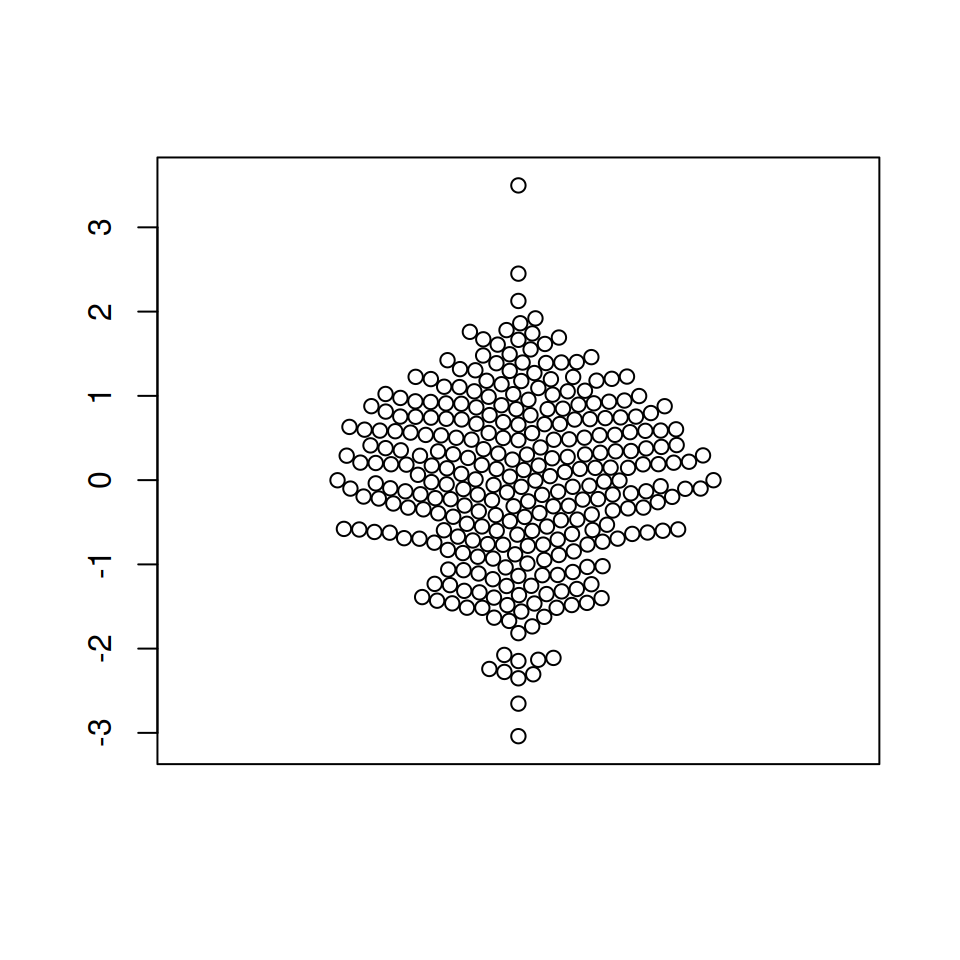

Basic bee swarm in R with beeswarm function

The plot can be customized the same way as other base R plots. Change the color of the points, the symbol and its size with col, pch and cex, respectively.

# install.packages("beeswarm")
library(beeswarm)

# Data generation
set.seed(1995)
x <- rnorm(300)

# Bee swarm plot
beeswarm(x,
         col = 2,   # Color
         pch = 18,  # Symbol
         cex = 1.5) # Size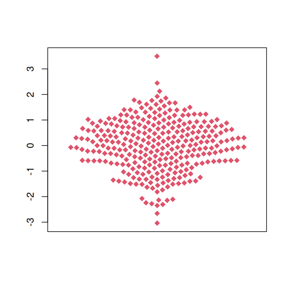

Bee swarm plot color customization

The plot can also be created in horizontal mode, setting vertical = FALSE or horizontal = TRUE.

# install.packages("beeswarm")
library(beeswarm)

# Data generation
set.seed(1995)
x <- rnorm(300)

# Horizontal bee swarm plot
beeswarm(x, col = 4,
         vertical = FALSE) #  Or horizontal = TRUE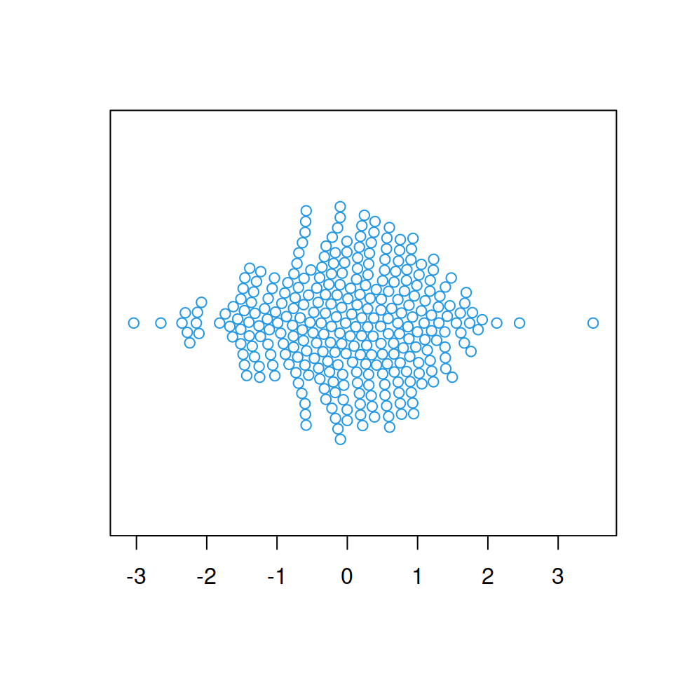

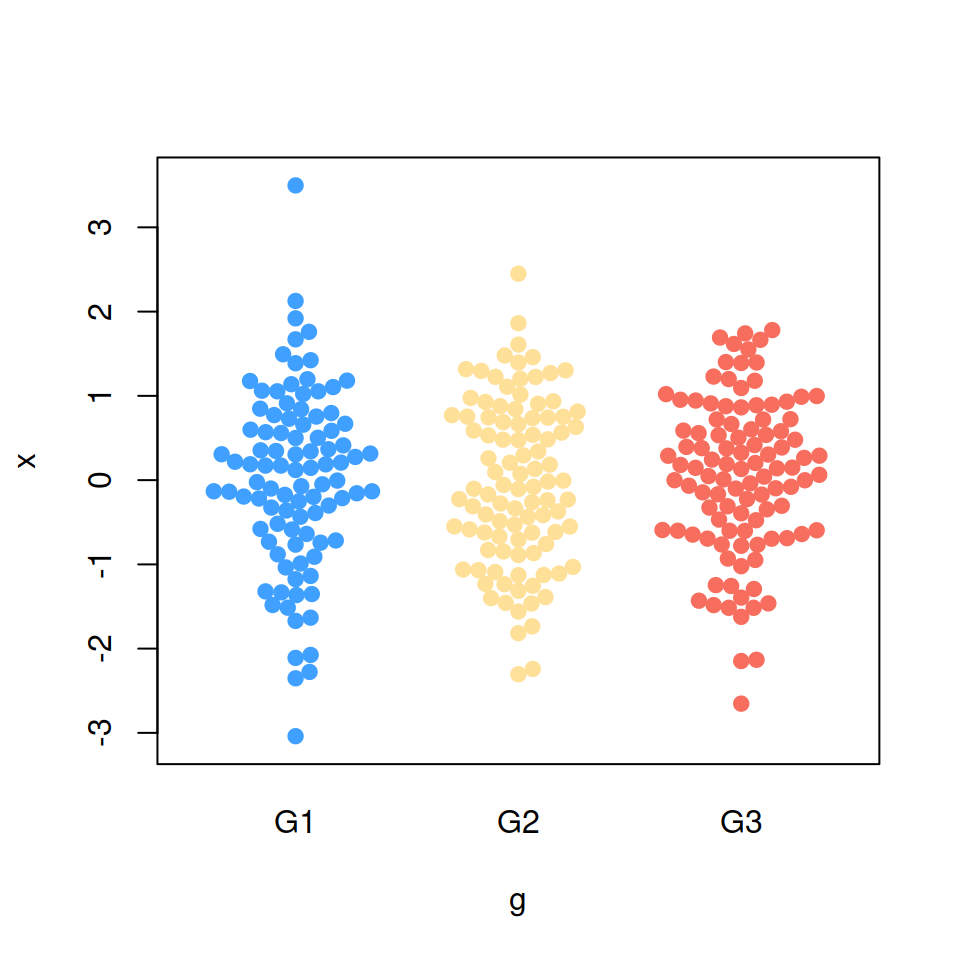
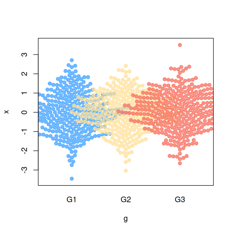
Horizontal beeswarm plot in R

Beeswarm by group

If you have a categorical variable representing groups it is possible to create a bee swarm plot by group based on the levels of that variable. For that purpose pass a formula to the function with the corresponding variables.

Beeswarm by group in R

# install.packages("beeswarm")
library(beeswarm)

# Data generation
set.seed(1995)
x <- rnorm(300)
g <- sample(c("G1", "G2", "G3"),
            size = 300, replace = TRUE)

# Bee swarm plot by group
beeswarm(x ~ g,
         pch = 19, 
         col = c("#3FA0FF", "#FFE099", "#F76D5E"))

If you have another categorical variable which represents some subgroups inside the main groups you can color each bee swarm with different colors representing that subcategories. Use the pwcol argument to indicate the colors. Alternatively, you can set the pch symbols with pwpch.

Bee swarm point wise

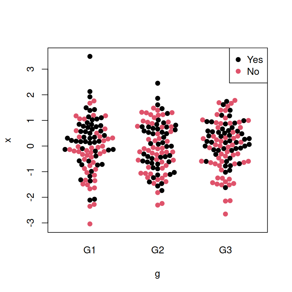
# install.packages("beeswarm")
library(beeswarm)

# Data generation
set.seed(1995)
x <- rnorm(300)
g <- sample(c("G1", "G2", "G3"),
            size = 300, replace = TRUE)
z <- as.numeric(factor(sample(c("Yes", "No"),
                size = 300, replace = TRUE)))

# Bee swarm plot by group
beeswarm(x ~ g,
         pch = 19, 
         pwcol = as.numeric(z))

# Legend
legend("topright", legend = c("Yes", "No"),
       col = 1:2, pch = 19)

Bee swarm plot methods

There are several methods available for arranging the data points. Each method uses a different algorithm ensuring that the data points are not overlapped.

“swarm” method (default)

This method places the points in increasing order.

# install.packages("beeswarm")
library(beeswarm)

# Data generation
set.seed(1995)
x <- rnorm(300)

# swarm method
beeswarm(x, col = 4, pch = 19,
         method = "swarm")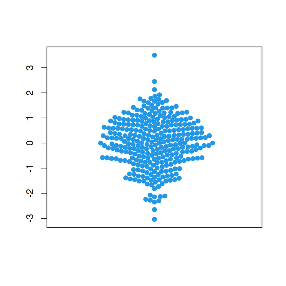

swarm arranging method

“center” method

The center method creates a symmetric swarm using a square grid.

# install.packages("beeswarm")
library(beeswarm)

# Data generation
set.seed(1995)
x <- rnorm(300)

# center method
beeswarm(x, col = 4, pch = 19,
         method = "center")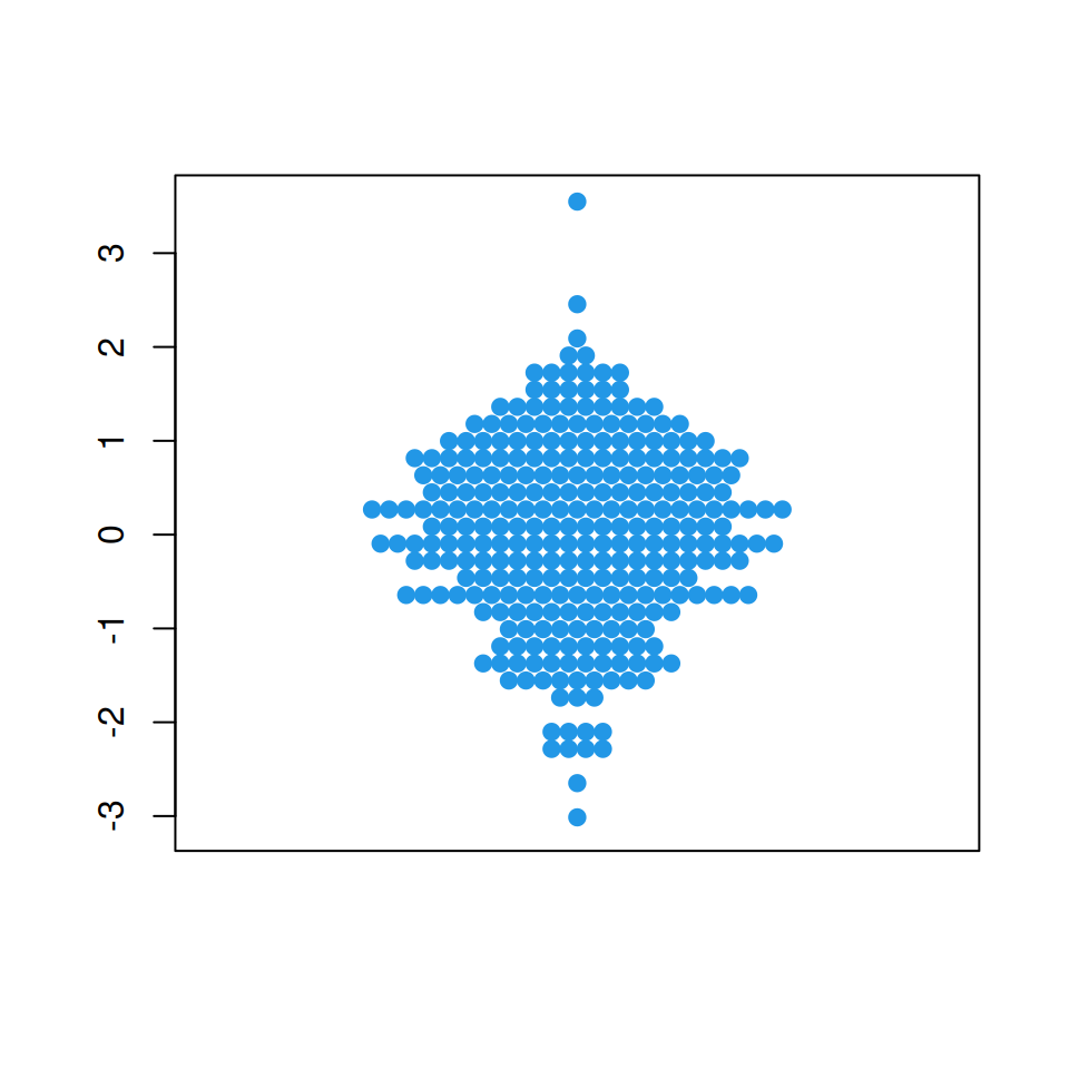

bee swarm center arranging method

“hex” method

This method uses a hexagonal grid to place the data points.

# install.packages("beeswarm")
library(beeswarm)

# Data generation
set.seed(1995)
x <- rnorm(300)

# hex method
beeswarm(x, col = 4, pch = 19,
         method = "hex")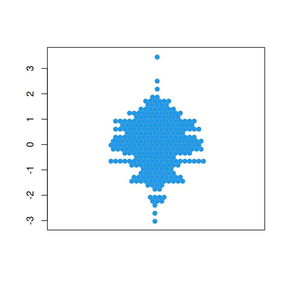

hex method for arranging points in the swarm plot

“square” method

The square method place the data points on a square grid.

# install.packages("beeswarm")
library(beeswarm)

# Data generation
set.seed(1995)
x <- rnorm(300)

# square method
beeswarm(x, col = 4, pch = 19,
         method = "square")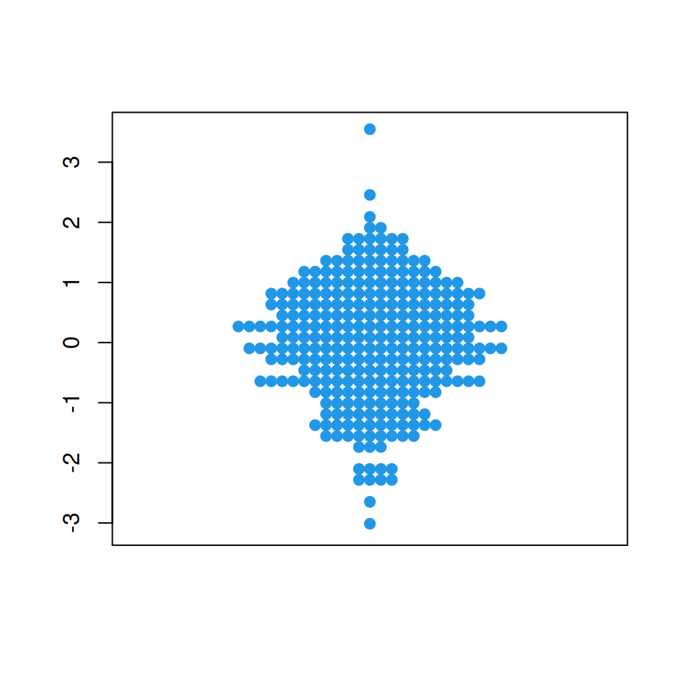

square arranging method in the R bee swarm plot

Bee swarm corral methods

If some observations are placed outside the plot area you can use a “corral” method, which will adjust that data points accordingly to the selected method.

Observations without corral method

Default

# install.packages("beeswarm")
library(beeswarm)

# Data generation
set.seed(1995)
x <- rnorm(1000)
g <- sample(c("G1", "G2", "G3"),
            size = 1000, replace = TRUE)

# Bee swarm plot by group
beeswarm(x ~ g, pch = 19, 
         col = c(rgb(0.25, 0.63, 1, 0.75),
                 rgb(1, 0.88, 0.6, 0.75),
                 rgb(0.97, 0.43, 0.37, 0.75)),
         corral = "none")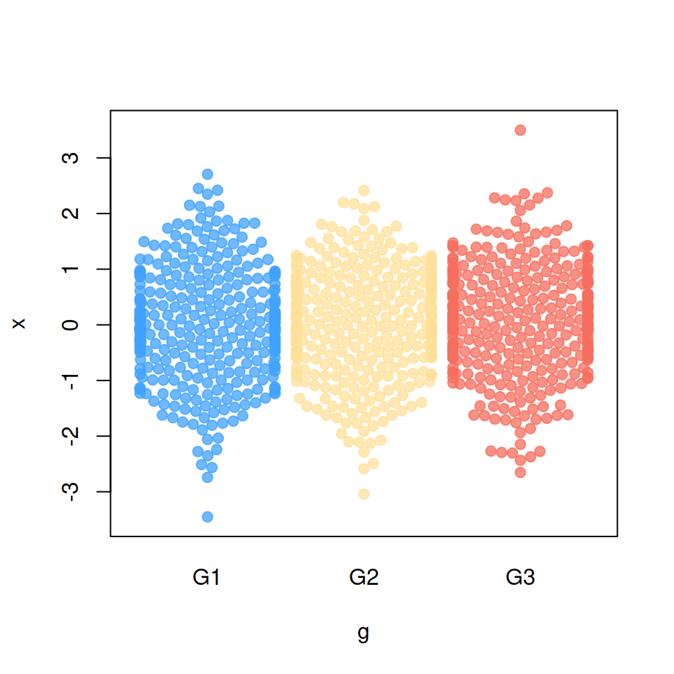

gutter corral method

“gutter” method

# install.packages("beeswarm")
library(beeswarm)

# Data generation
set.seed(1995)
x <- rnorm(1000)
g <- sample(c("G1", "G2", "G3"),
            size = 1000, replace = TRUE)

# Bee swarm plot by group
beeswarm(x ~ g, pch = 19, 
         col = c(rgb(0.25, 0.63, 1, 0.75),
                 rgb(1, 0.88, 0.6, 0.75),
                 rgb(0.97, 0.43, 0.37, 0.75)),
         corral = "gutter")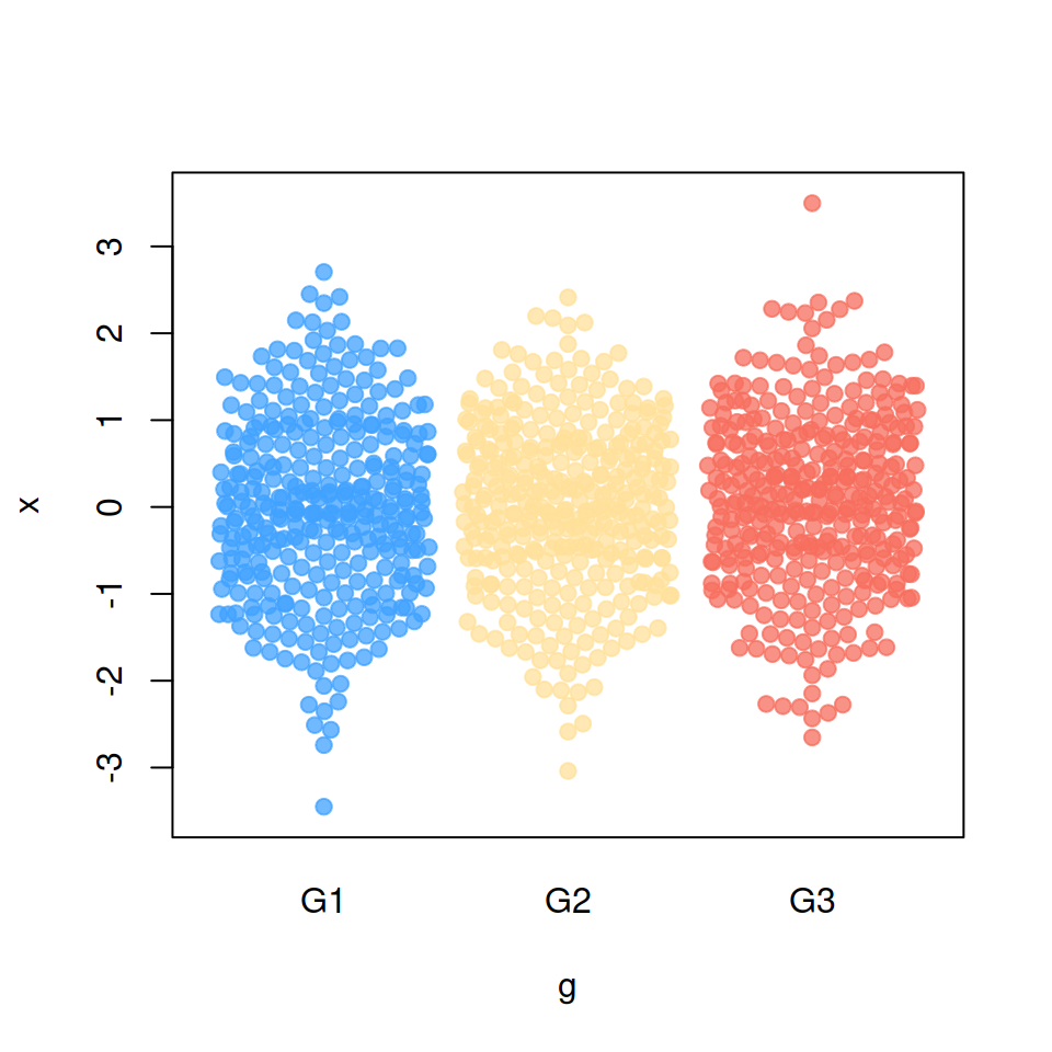

wrap bee swarm plot corral method

“wrap” method

# install.packages("beeswarm")
library(beeswarm)

# Data generation
set.seed(1995)
x <- rnorm(1000)
g <- sample(c("G1", "G2", "G3"),
            size = 1000, replace = TRUE)

# Bee swarm plot by group
beeswarm(x ~ g, pch = 19, 
         col = c(rgb(0.25, 0.63, 1, 0.75),
                 rgb(1, 0.88, 0.6, 0.75),
                 rgb(0.97, 0.43, 0.37, 0.75)),
         corral = "wrap")

random corral method

“random” method

# install.packages("beeswarm")
library(beeswarm)

# Data generation
set.seed(1995)
x <- rnorm(1000)
g <- sample(c("G1", "G2", "G3"),
            size = 1000, replace = TRUE)

# Bee swarm plot by group
beeswarm(x ~ g, pch = 19, 
         col = c(rgb(0.25, 0.63, 1, 0.75),
                 rgb(1, 0.88, 0.6, 0.75),
                 rgb(0.97, 0.43, 0.37, 0.75)),
         corral = "random")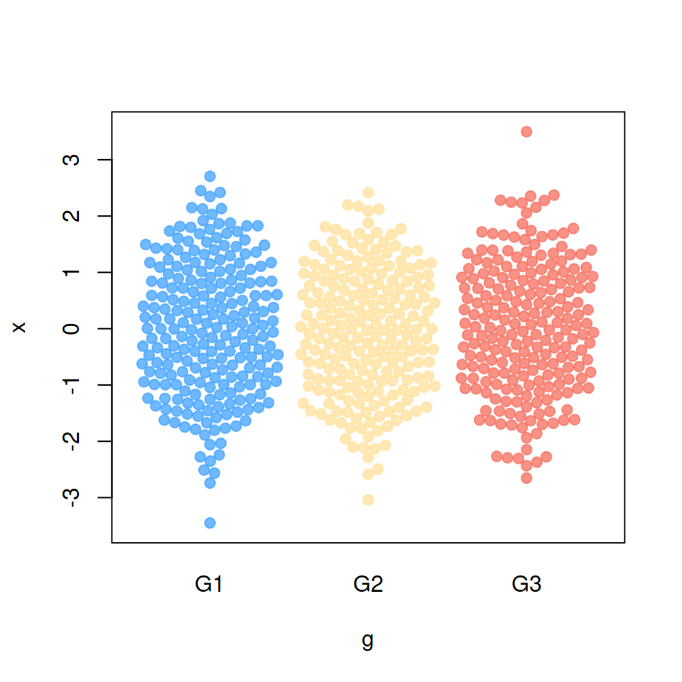

omit corral method R bee swarm

“omit” method

# install.packages("beeswarm")
library(beeswarm)

# Data generation
set.seed(1995)
x <- rnorm(1000)
g <- sample(c("G1", "G2", "G3"),
            size = 1000, replace = TRUE)

# Bee swarm plot by group
beeswarm(x ~ g, pch = 19, 
         col = c(rgb(0.25, 0.63, 1, 0.75),
                 rgb(1, 0.88, 0.6, 0.75),
                 rgb(0.97, 0.43, 0.37, 0.75)),
         corral = "omit")

Bee swarm side

It is possible to display only one side of the bee swarm plot. Set side = -1 to add the points on the left (or downwards).

# install.packages("beeswarm")
library(beeswarm)

# Data generation
set.seed(1995)
x <- rnorm(300)
g <- sample(c("G1", "G2", "G3"),
            size = 300, replace = TRUE)

# Left side
beeswarm(x ~ g, pch = 19, 
         col = c("#3FA0FF", "#FFE099", "#F76D5E"),
         side = -1)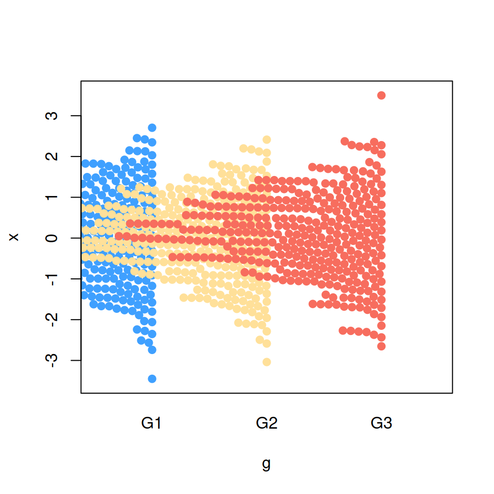

Bee swarm left side

Set side = 1 so the jittering is performed to the right or upwards.

# install.packages("beeswarm")
library(beeswarm)

# Data generation
set.seed(1995)
x <- rnorm(300)
g <- sample(c("G1", "G2", "G3"),
            size = 300, replace = TRUE)

# Right side
beeswarm(x ~ g, pch = 19, 
         col = c("#3FA0FF", "#FFE099", "#F76D5E"),
         side = 1)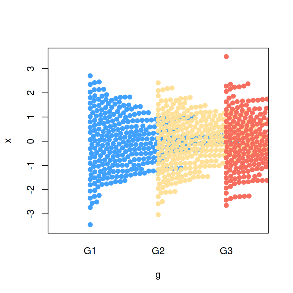

beeswarm plot right side

Bee swarm priority

When method = "swarm" you can modify the order used to perform the priority layout. The default method is "ascending" and the other possible values are displayed below. Recall to type ?beeswarm for more information about these methods.

Descending priority layout in R beeswarm function

“descending” priority

# install.packages("beeswarm")
library(beeswarm)

# Data generation
set.seed(1995)
x <- rnorm(300)
g <- sample(c("G1", "G2", "G3"),
            size = 300, replace = TRUE)

# Bee swarm with descending priority
beeswarm(x ~ g, pch = 19, 
         col = c("#3FA0FF", "#FFE099", "#F76D5E"),
         priority = "descending")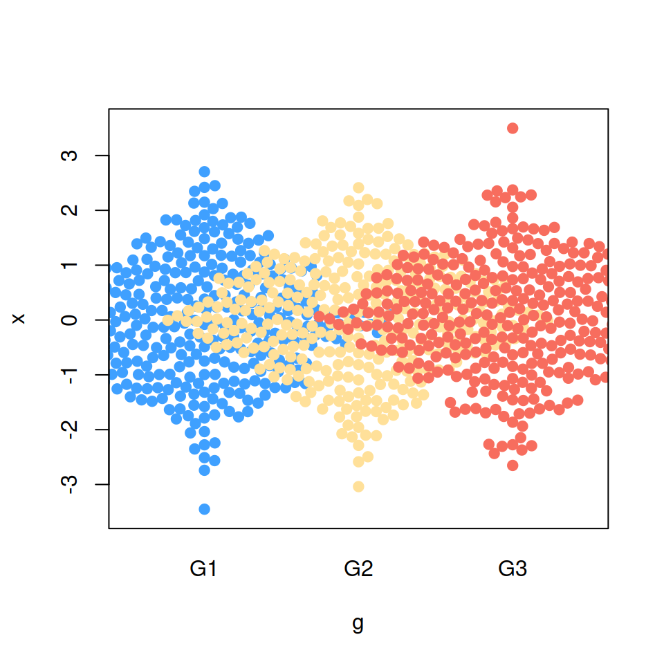

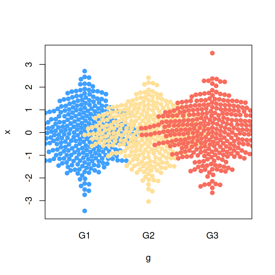
beeswarm package with random priority

“random” priority

# install.packages("beeswarm")
library(beeswarm)

# Data generation
set.seed(1995)
x <- rnorm(300)
g <- sample(c("G1", "G2", "G3"),
            size = 300, replace = TRUE)

# Bee swarm with random priority
beeswarm(x ~ g, pch = 19, 
         col = c("#3FA0FF", "#FFE099", "#F76D5E"),
         priority = "random")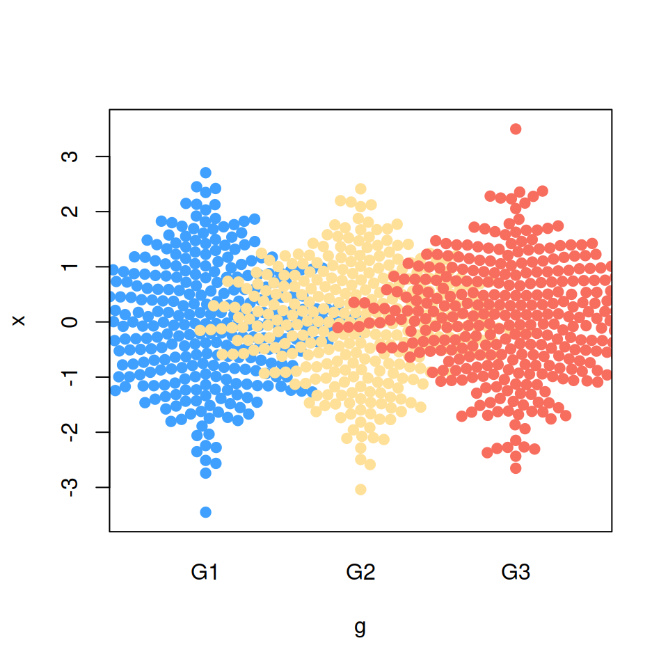

density priority swarm method

“density” priority

# install.packages("beeswarm")
library(beeswarm)

# Data generation
set.seed(1995)
x <- rnorm(300)
g <- sample(c("G1", "G2", "G3"),
            size = 300, replace = TRUE)

# Bee swarm with density priority
beeswarm(x ~ g, pch = 19, 
         col = c("#3FA0FF", "#FFE099", "#F76D5E"),
         priority = "density")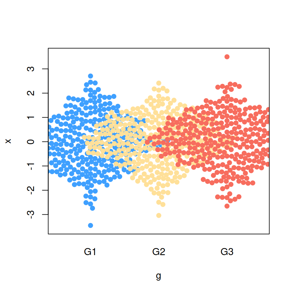

none priority swarm method

“none” priority

# install.packages("beeswarm")
library(beeswarm)

# Data generation
set.seed(1995)
x <- rnorm(300)
g <- sample(c("G1", "G2", "G3"),
            size = 300, replace = TRUE)

# Bee swarm with none priority
beeswarm(x ~ g, pch = 19, 
         col = c("#3FA0FF", "#FFE099", "#F76D5E"),
         priority = "none")