Density plot in ggplot2 with geom_density
Given a continuous variable you can create a density plot in ggplot2 with geom_density.
# install.packages("ggplot2")
library(ggplot2)

# Data
set.seed(14012021)
x <- rnorm(200, mean = 4)
df <- data.frame(x)

# Basic density plot in ggplot2
ggplot(df, aes(x = x)) +
  geom_density()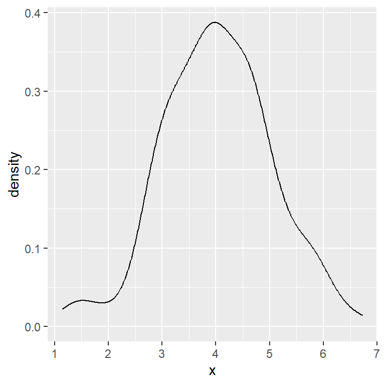
The curve can be customized in several ways, such as changing its color, width or type.
# install.packages("ggplot2")
library(ggplot2)

# Data
set.seed(14012021)
x <- rnorm(200, mean = 4)
df <- data.frame(x)

# Density plot in ggplot2
ggplot(df, aes(x = x)) +
  geom_density(color = 4,
               lwd = 1,
               linetype = 1)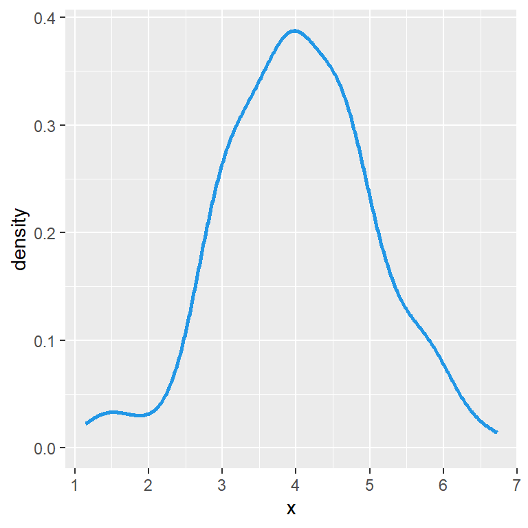
You can also fill the area and change its transparency with fill and alpha, respectively.
# install.packages("ggplot2")
library(ggplot2)

# Data
set.seed(14012021)
x <- rnorm(200, mean = 4)
df <- data.frame(x)

# Density plot in ggplot2
ggplot(df, aes(x = x)) +
  geom_density(color = 4,
               fill = 4,
               alpha = 0.25)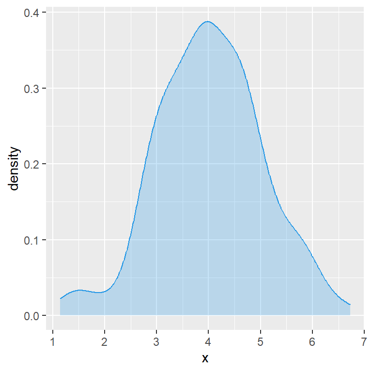
Smoothing parameter selection
When calculating a kernel density estimate a smoothing parameter (also known as bandwidth) must be selected. A big bandwidth will create a very smoothed curve, while a small bandwidth will create a sharpened curve.
The default method used for calculating the bandwidth is called rule-of-thumb, but you can choose between other options, use a bandwidth multiplier or the value you desire, as shown in the following examples.
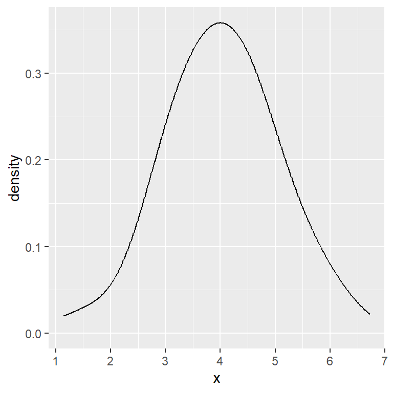
Bandwidth multiplier
# install.packages("ggplot2")
library(ggplot2)

# Data
set.seed(14012021)
x <- rnorm(200, mean = 4)
df <- data.frame(x)

# Density plot, bandwidth multiplier
ggplot(df, aes(x = x)) +
  geom_density(adjust = 1.75)
Scott bandwidth (factor 1.06)
# install.packages("ggplot2")
library(ggplot2)

# Data
set.seed(14012021)
x <- rnorm(200, mean = 4)
df <- data.frame(x)

# Density plot, Scott bandwidth
ggplot(df, aes(x = x)) +
  geom_density(bw = "nrd")
Unbiased cross validation method
# install.packages("ggplot2")
library(ggplot2)

# Data
set.seed(14012021)
x <- rnorm(200, mean = 4)
df <- data.frame(x)

# Unbiased cross validation bandwidth
ggplot(df, aes(x = x)) +
  geom_density(bw = "ucv")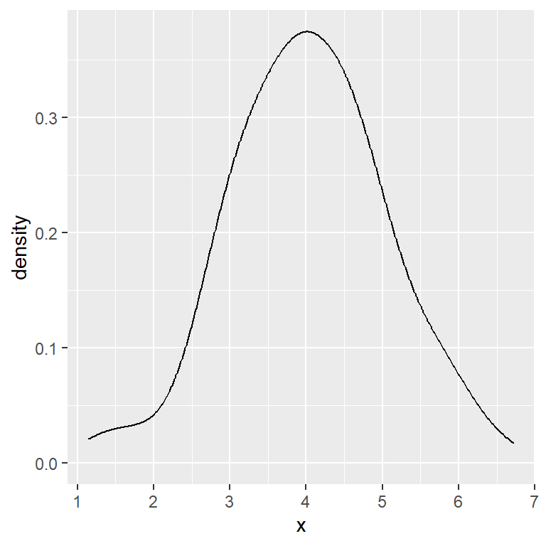
Biased cross validation method
# install.packages("ggplot2")
library(ggplot2)

# Data
set.seed(14012021)
x <- rnorm(200, mean = 4)
df <- data.frame(x)

# Biased cross validation bandwidth
ggplot(df, aes(x = x)) +
  geom_density(bw = "bcv")
Sheather & Jones method
# install.packages("ggplot2")
library(ggplot2)

# Data
set.seed(14012021)
x <- rnorm(200, mean = 4)
df <- data.frame(x)

# SJ bandwidth
ggplot(df, aes(x = x)) +
  geom_density(bw = "SJ")
Kernel selection
The kernel used can also be changed with kernel argument. The possible options are "gaussian" (default), "rectangular", "triangular", "epanechnikov", "biweight", "cosine" and "optcosine".
Below you can see an example which uses a rectangular kernel instead of a gaussian kernel. The decision about which kernel to use will depend on your data.
Rectangular kernel
# install.packages("ggplot2")
library(ggplot2)

# Data
set.seed(14012021)
x <- rnorm(200, mean = 4)
df <- data.frame(x)

# Custom kernel
ggplot(df, aes(x = x)) +
  geom_density(kernel = "rectangular")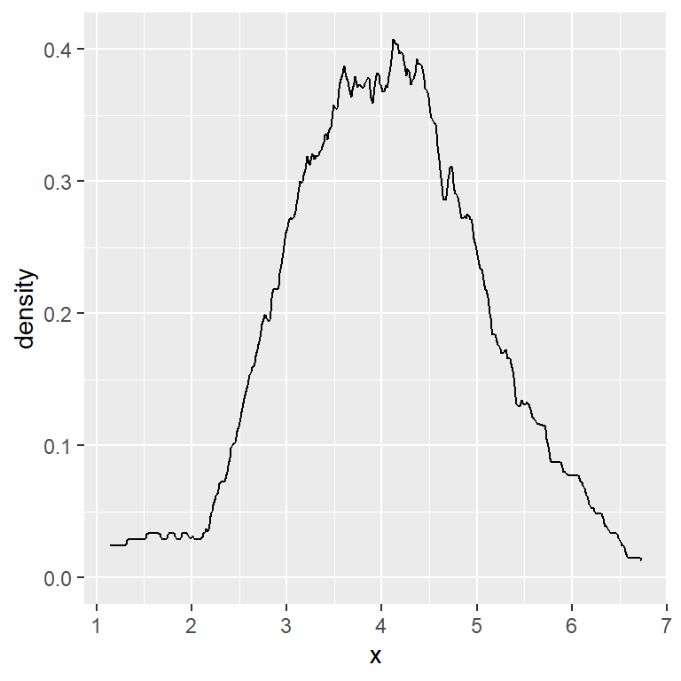

Master Statistics
Learn statistics from the basics to advanced techniques, clearly explained
Go to site