ggforce: Extensions for ggplot2

Package

Author

Thomas Lin Pedersen

Sample data

ggforce is a ggplot2 extension by Thomas Lin Pedersen, the current maintainer of ggplot2. It adds new geoms, stats and facets that complement the core package. We use the iris dataset throughout this post.

# install.packages("ggforce")
library(ggplot2)
library(ggforce)

head(iris, 6)

`geom_sina()`

geom_sina() is a variation of jitter that constrains points within the violin shape, combining the density information of a violin with the individual points of a jitter plot. Layer it on top of geom_violin() for a complete view of the distribution.

# install.packages("ggforce")
library(ggplot2)
library(ggforce)

ggplot(iris, aes(x = Species,
                 y = Sepal.Length,
                 color = Species)) +
  geom_violin(alpha = 0.2) +
  geom_sina() +
  theme_minimal()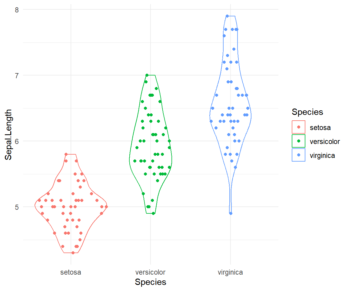

Sina plot with ggforce geom_sina in R

`geom_mark_ellipse()`

Mark groups with ellipses using ggforce geom_mark_ellipse in R

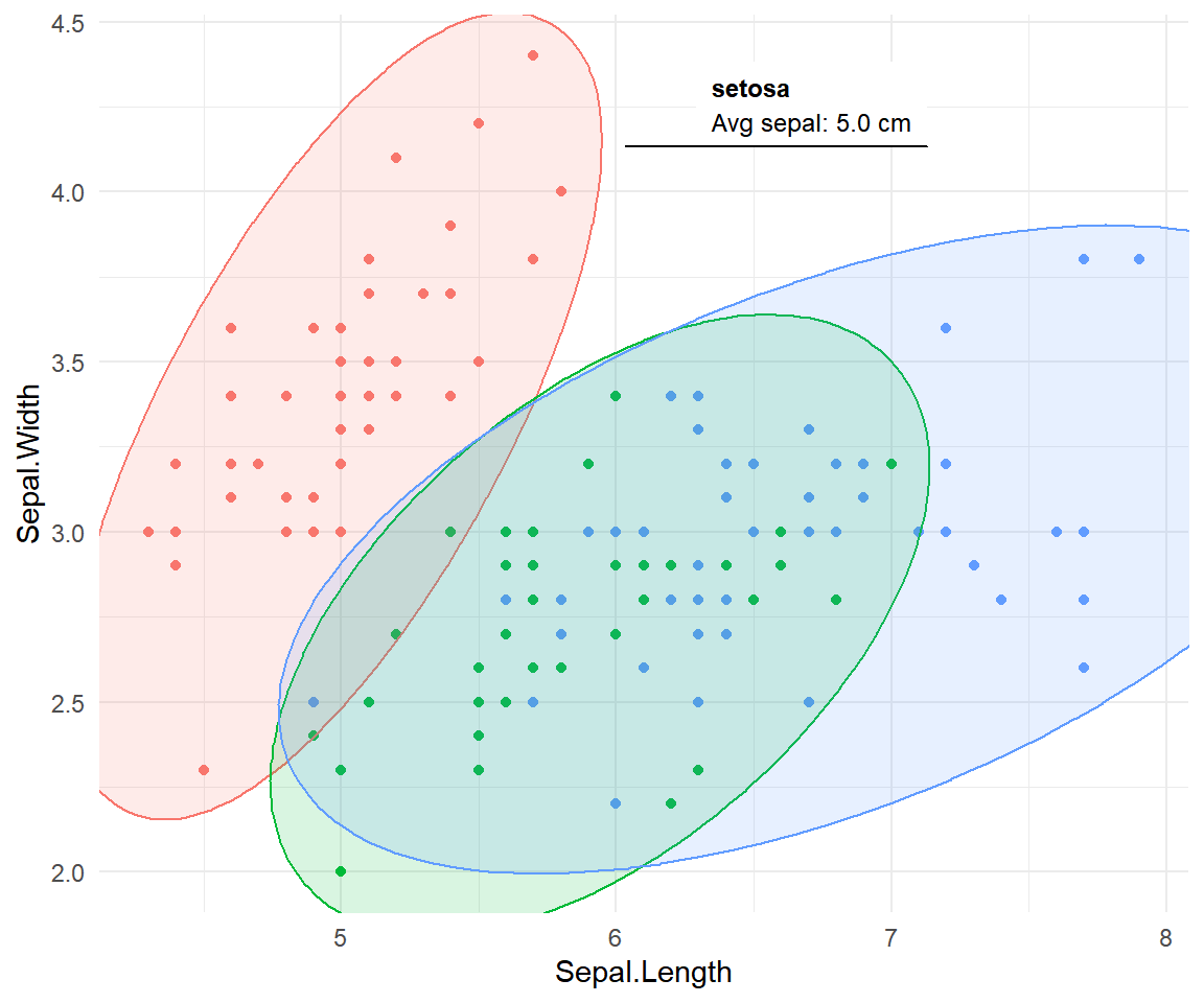
geom_mark_ellipse() draws an ellipse around each group. Map label and optionally description inside aes() to add annotated callouts. Control text size with label.fontsize and padding with expand.

# install.packages("ggforce")
library(ggplot2)
library(ggforce)

ggplot(iris, aes(x = Sepal.Length,
                 y = Sepal.Width,
                 color = Species)) +
  geom_point() +
  geom_mark_ellipse(
    aes(fill = Species, label = Species,
        description = desc),
    alpha = 0.15, label.fontsize = 9) +
  theme_minimal() +
  theme(legend.position = "none")

`geom_mark_hull()`

geom_mark_hull() draws a concave hull that fits the boundary tightly around the actual data points. The concavity argument controls the tightness: lower values produce a more concave boundary, higher values tend toward a convex hull.

# install.packages("ggforce")
library(ggplot2)
library(ggforce)

ggplot(iris, aes(x = Sepal.Length,
                 y = Sepal.Width,
                 color = Species)) +
  geom_point() +
  geom_mark_hull(
    aes(fill = Species, label = Species),
    alpha = 0.15, concavity = 2) +
  theme_minimal() +
  theme(legend.position = "none")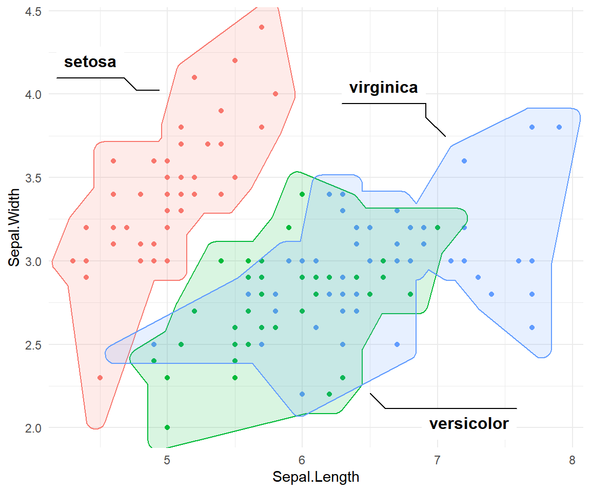

Mark groups with concave hull using ggforce geom_mark_hull in R

`geom_mark_rect()`

Mark groups with bounding rectangles using ggforce geom_mark_rect in R

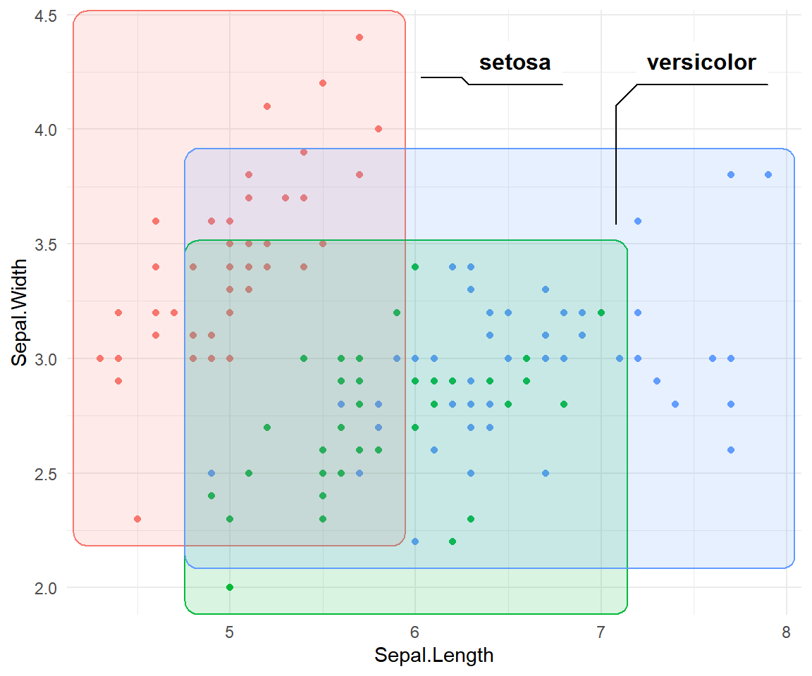
geom_mark_rect() draws the smallest axis-aligned bounding rectangle around each group. It is the most compact of the three mark geoms and works well when groups are roughly rectangular in shape. It accepts the same label, description and styling arguments as the other mark geoms.

# install.packages("ggforce")
library(ggplot2)
library(ggforce)

ggplot(iris, aes(x = Sepal.Length,
                 y = Sepal.Width,
                 color = Species)) +
  geom_point() +
  geom_mark_rect(
    aes(fill  = Species,
        label = Species),
    alpha = 0.15) +
  theme_minimal() +
  theme(legend.position = "none")

`geom_parallel_sets()`

geom_parallel_sets() draws a Sankey-like diagram showing how observations distribute across multiple categorical variables. First reshape the data with gather_set_data(), then use three companion geoms: geom_parallel_sets() for the ribbons, geom_parallel_sets_axes() for the axis bars and geom_parallel_sets_labels() for the labels.

# install.packages("ggforce")
library(ggplot2)
library(ggforce)

df_long <- gather_set_data(
  iris[, c("Species", "Sepal.Size")], 1:2)

ggplot(df_long, aes(x = x, id = id,
                    split = y, value = 1)) +
  geom_parallel_sets(aes(fill = Species), alpha = 0.4) +
  geom_parallel_sets_axes(axis.width = 0.1) +
  geom_parallel_sets_labels(colour = "white") +
  theme_void()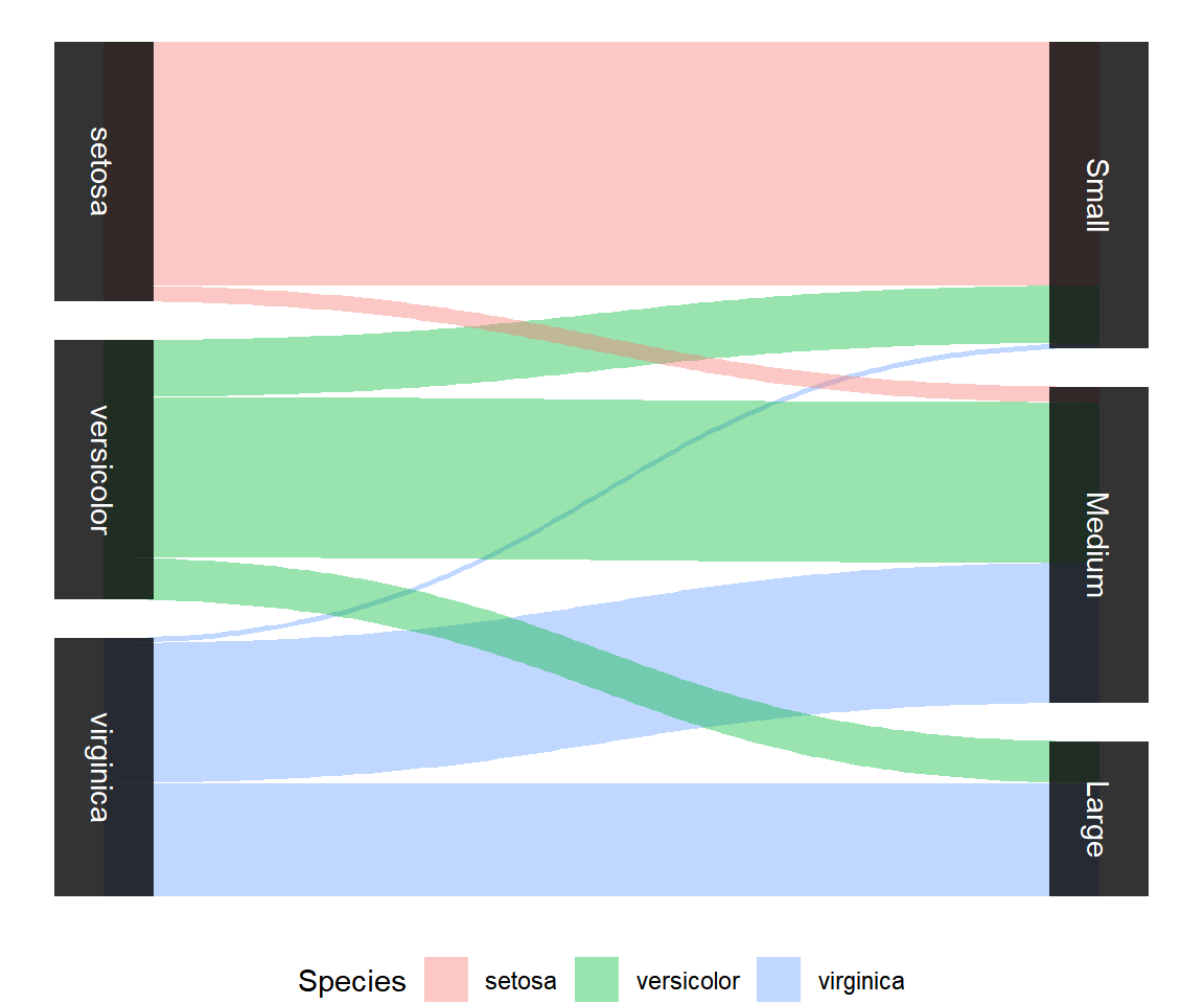

Parallel sets diagram with ggforce geom_parallel_sets in R

`facet_wrap_paginate()`

Paginated facets with ggforce facet_wrap_paginate in R

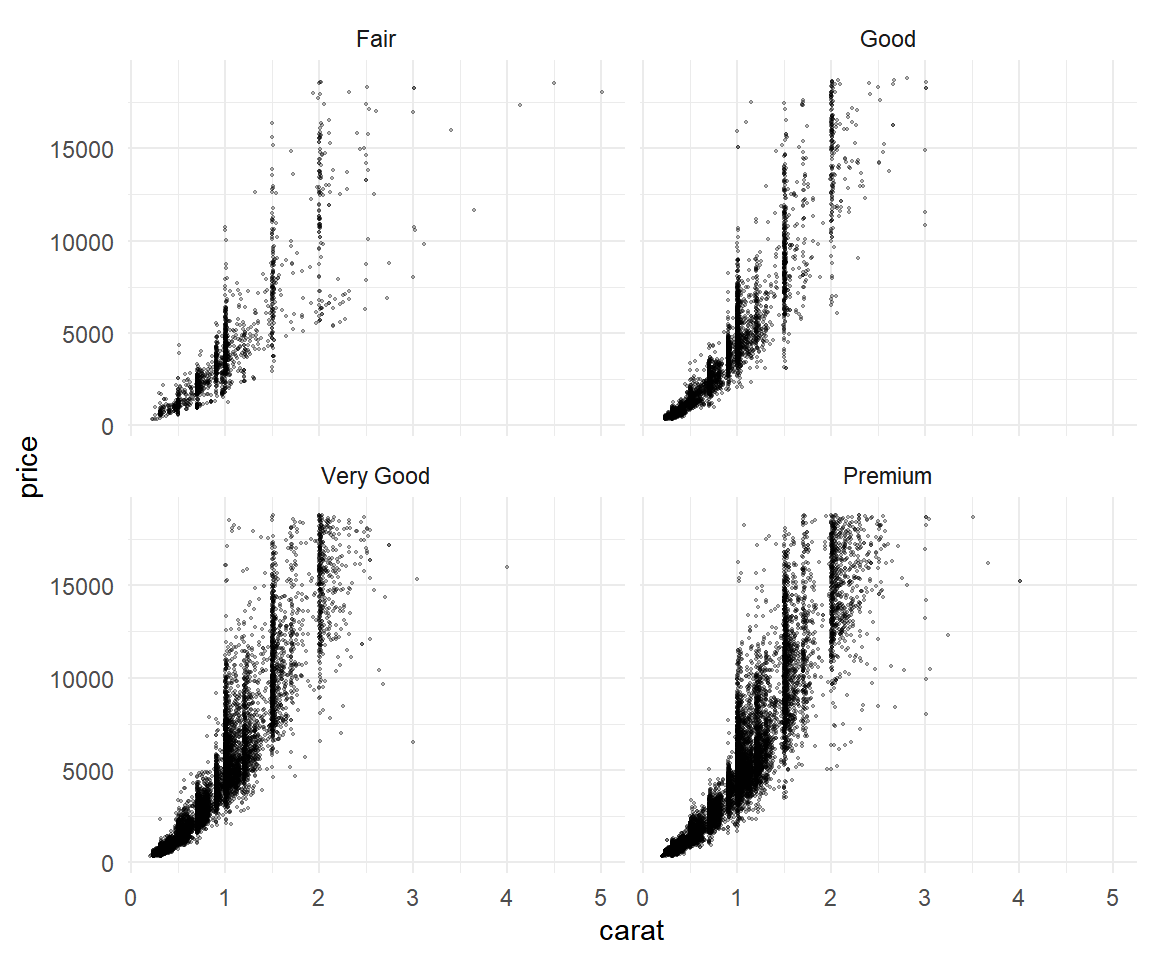
facet_wrap_paginate() works like facet_wrap() but splits the panels across pages. Set ncol and nrow to define the grid per page, then change page to render a different subset. Use n_pages() on the same call to find the total number of pages.

# install.packages("ggforce")
library(ggplot2)
library(ggforce)

ggplot(diamonds, aes(x = carat, y = price)) +
  geom_point(alpha = 0.3, size = 0.3) +
  facet_wrap_paginate(~ cut,
                      ncol = 2, nrow = 2,
                      page = 1) +
  theme_minimal()