Kernel density plot in R

Kernel density estimation

In order to create a kernel density plot you will need to estimate the kernel density. For that purpose you can use the density function and then pass the density object to the plot function.

# Data
set.seed(14012021)
data <- rnorm(200, mean = 4)

# Kernel density estimation
d <- density(data)

# Kernel density plot
plot(d, lwd = 2, main = "Default kernel density plot")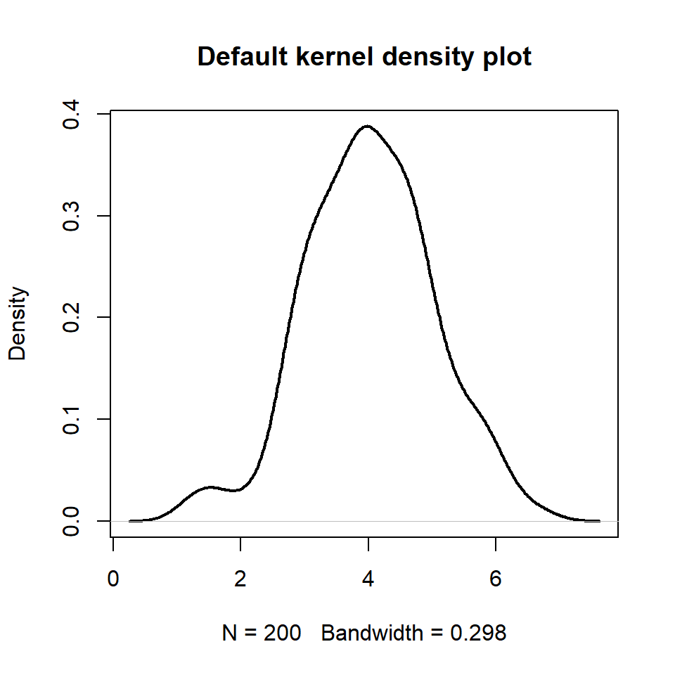

Kernel density plot in R

Kernel selection

The kernel argument of the density function uses the gaussian kernel by default (kernel = "gaussian"), but there are more kernel types available, such as "rectangular", "triangular", "epanechnikov", "biweight", "cosine" and "optcosine". The selection will depend on your data, but in most scenarios the default value is the most recommended.

Rectangular kernel plot in R

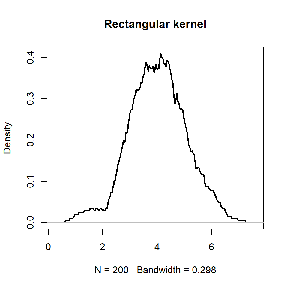
Rectangular kernel

# Data
set.seed(14012021)
data <- rnorm(200, mean = 4)

# Kernel density estimation
d <- density(data,
             kernel = "rectangular")

# Kernel density plot
plot(d, lwd = 2, main = "Rectangular kernel")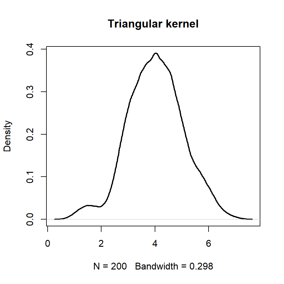

Triangular kernel density plot

Triangular kernel

# Data
set.seed(14012021)
data <- rnorm(200, mean = 4)

# Kernel density estimation
d <- density(data,
             kernel = "triangular")

# Kernel density plot
plot(d, lwd = 2, main = "Triangular kernel")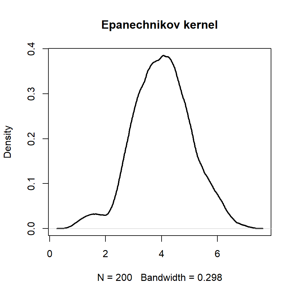

Epanechnikov kernel density in R

Epanechnikov kernel

# Data
set.seed(14012021)
data <- rnorm(200, mean = 4)

# Kernel density estimation
d <- density(data,
             kernel = "epanechnikov")

# Kernel density plot
plot(d, lwd = 2, main = "Epanechnikov kernel")

Biweight kernel in R

Biweight kernel

# Data
set.seed(14012021)
data <- rnorm(200, mean = 4)

# Kernel density estimation
d <- density(data,
             kernel = "biweight")

# Kernel density plot
plot(d, lwd = 2, main = "Biweight kernel")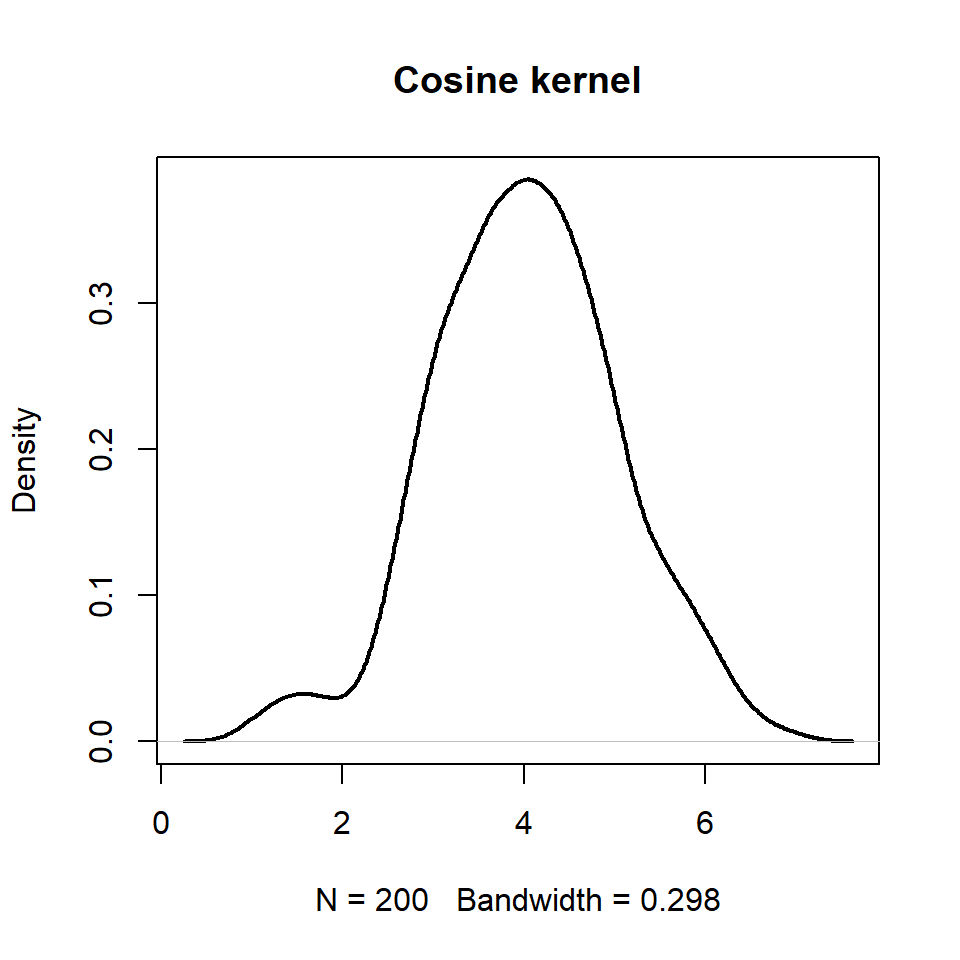

Cosine kernel density estimation plot

Cosine kernel

# Data
set.seed(14012021)
data <- rnorm(200, mean = 4)

# Kernel density estimation
d <- density(data,
             kernel = "cosine")

# Kernel density plot
plot(d, lwd = 2, main = "Cosine kernel")

Bandwidth selection

The bw argument of the density function allows changing the smoothing bandwidth used. You can pass either a value or a string giving a selection rule or a function. The default value is "nrd0" (or bw.nrd0(.)), which implements a rule-of-thumb approach. Other available options are:

Rule-of-thumb variation given by Scott (1992)

"nrd" or bw.nrd(.)

# Data
set.seed(14012021)
data <- rnorm(200, mean = 4)

# Kernel density estimation
d <- density(data,
             bw = "nrd")

# Kernel density plot
plot(d, lwd = 2, main = "nrd bandwidth")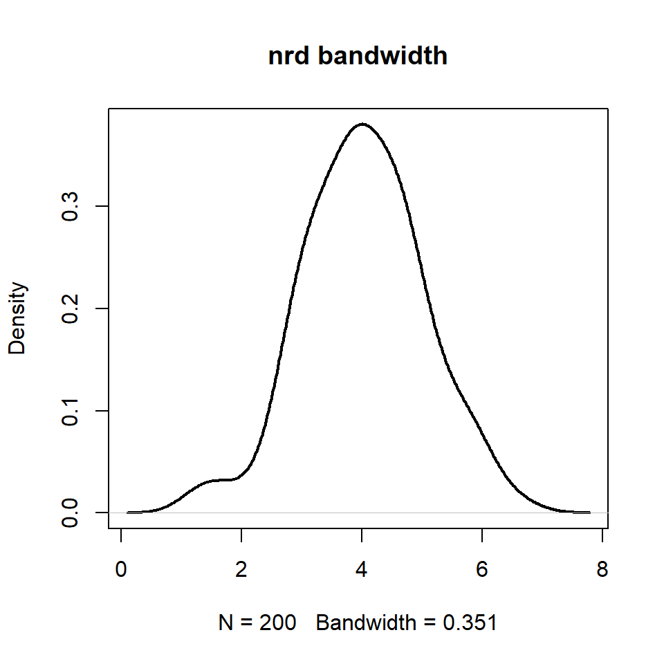

Rule of thumb bandwidth selection by Scott

Unbiased cross-validation

"ucv" or bw.ucv(.)

# Data
set.seed(14012021)
data <- rnorm(200, mean = 4)

# Kernel density estimation
d <- density(data,
             bw = "ucv")

# Kernel density plot
plot(d, lwd = 2, main = "ucv bandwidth")

Unbiased cross validation bandwidth selection in R

Biased cross-validation

"bcv" or bw.bcv(.)

# Data
set.seed(14012021)
data <- rnorm(200, mean = 4)

# Kernel density estimation
d <- density(data,
             bw = "bcv")

# Kernel density plot
plot(d, lwd = 2, main = "bcv bandwidth")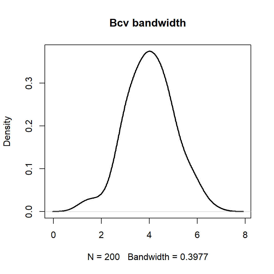

Biased cross validation method for selecting the density bandwidth parameter

Methods by Sheather & Jones (1991)

"SJ" or bw.SJ(.)

# Data
set.seed(14012021)
data <- rnorm(200, mean = 4)

# Kernel density estimation
d <- density(data,
             bw = "SJ")

# Kernel density plot
plot(d, lwd = 2, main = "SJ bandwidth")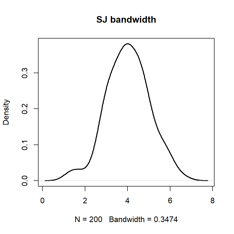

Sheather and Jones methods for bandwidth selection in R

The bandwidth must be chosen carefully. A small bandwidth will create a very overfitted curve while a too big bandwidth will create an oversmoothed curve.