Scatter plot based on a model
You can create a scatter plot based on a theoretical model and add it to the plot with the lines function. Consider the example of the following block of code as illustration.
# Data. Model: Y = X ^ 2
set.seed(54)
x <- seq(0, 10, by = 0.05)
y <- x ^ 2 + rnorm(length(x), sd = 20)

# Scatter plot and underlying model
plot(x, y, pch = 16)
lines(x, x ^ 2, col = 2, lwd = 3)

# Text
text(2, 70, expression(Y == X ^ 2))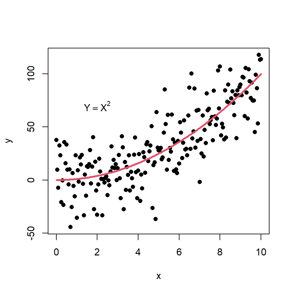
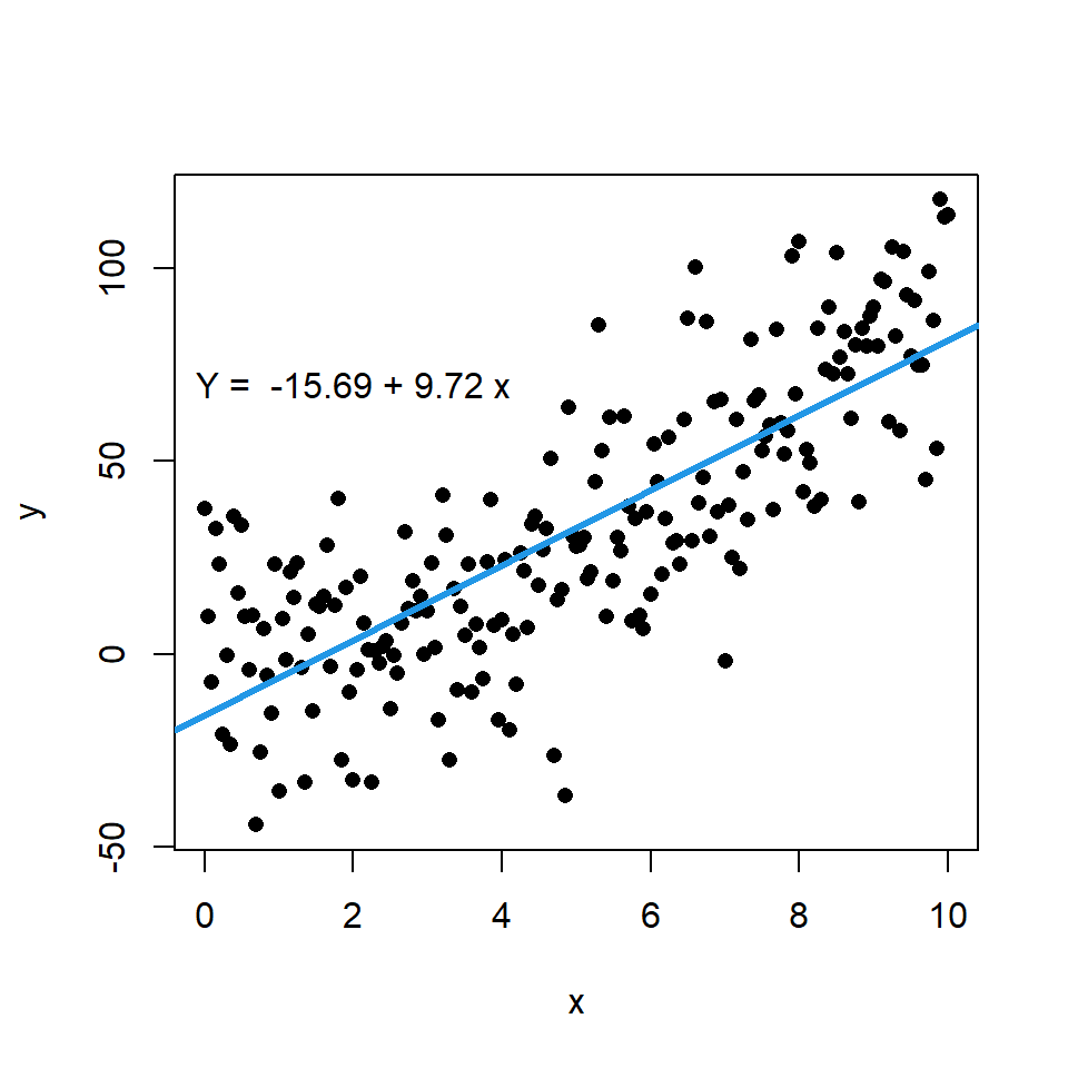
Scatter plot with linear regression
You can add a regression line to a scatter plot passing a lm object to the abline function. Recall that coef returns the coefficients of an estimated linear model.
# Data. Model: Y = X ^ 2
set.seed(54)
x <- seq(0, 10, by = 0.05)
y <- x ^ 2 + rnorm(length(x), sd = 20)

# Linear model
model <- lm(y ~ x)

# Scatter plot and linear regression line
plot(x, y, pch = 16)
abline(model, col = 4, lwd = 3)

# Text
coef <- round(coef(model), 2)
text(2, 70,  paste("Y = ", coef[1], "+", coef[2], "x"))
In addition, if you want you can display the error terms or residuals between actual and estimated values by using the segments function. For that purpose you can input the variable x to the x0 and x1 arguments, the variable y to y0 and the estimate of the model, which is calculated with predict, to y1.
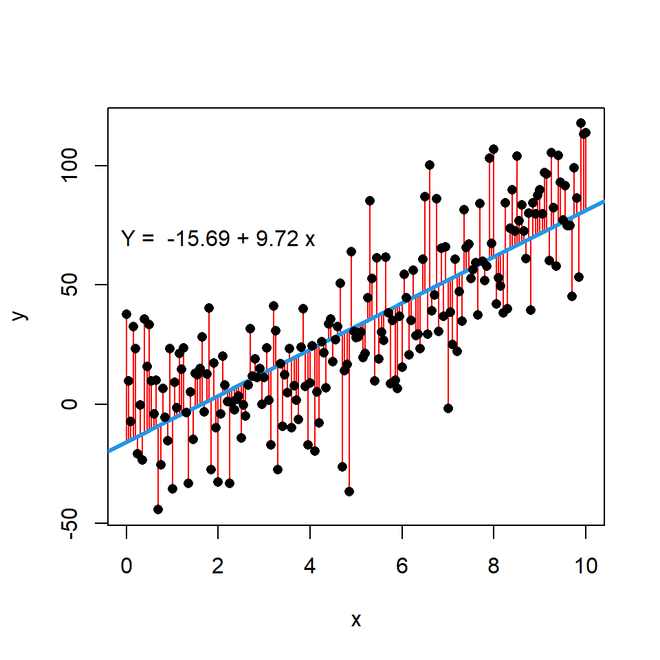
# Data. Model: Y = X ^ 2
set.seed(54)
x <- seq(0, 10, by = 0.05)
y <- x ^ 2 + rnorm(length(x), sd = 20)

# Linear model
modelo <- lm(y ~ x)

# Scatter plot and linear regression line
plot(x, y, pch = 16)

# Segments with error terms
segments(x0 = x, x1 = x, y0 = y, y1 = predict(modelo),
         lwd = 1, col = "red")

# Regression line
abline(modelo, col = 4, lwd = 3)

# Paint the points again over the segments
points(x, y, pch = 16)

# Text
coef <- round(coef(modelo), 2)
text(2, 70,  paste("Y = ", coef[1], "+", coef[2], "x"))
Scatter plot with LOWESS regression curve
The LOWESS smoother uses locally-weighted polynomial regression. This non-parametric regression can be estimated with lowess function.
# Data. Model: Y = X ^ 2
set.seed(54)
x <- seq(0, 10, by = 0.05)
y <- x ^ 2 + rnorm(length(x), sd = 20)

# Scatter plot and LOWESS regression curve
plot(x, y, pch = 16)
lines(lowess(x, y), col = 3, lwd = 3)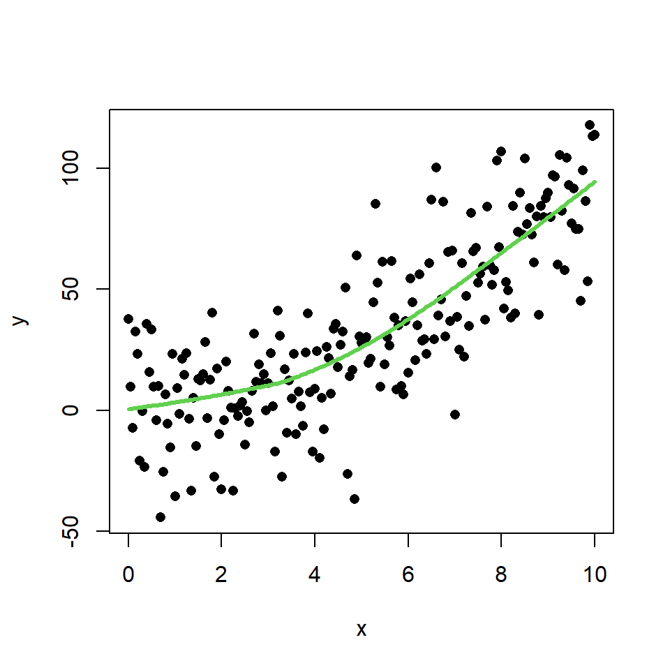
In this scenario, this method makes a better approximation of the theoretical model than the linear regression. You can check it comparing the theoretical model and the estimate of the LOWESS smoother:
# Data. Model: Y = X ^ 2
set.seed(54)
x <- seq(0, 10, by = 0.05)
y <- x ^ 2 + rnorm(length(x), sd = 20)

plot(x, y, pch = 16)

# Estimated model
lines(lowess(x, y), col = 3, lwd = 3)

# Theoretical model
lines(x, x ^ 2, col = 2, lwd = 3)

# Legend
legend(x = "topleft", # Position
       legend = c("LOWESS", "Theoretical"), # Texts
       lty = 1,       # Line types
       col = c(3, 2), # Colors
       lwd = 2)       # Line width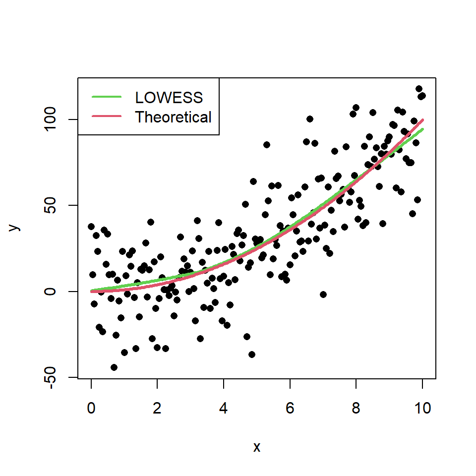

Master Statistics
Learn statistics from the basics to advanced techniques, clearly explained
Go to site