Coordinate systems in ggplot2 can be divided into two categories: linear (coord_cartesian, coord_fixed, coord_flip) and non-linear (coord_trans, coord_polar, coord_quickmap, coord_map) coordinate systems. These systems will be reviewed in this tutorial.
Cartesian coordiantes with coord_cartesian
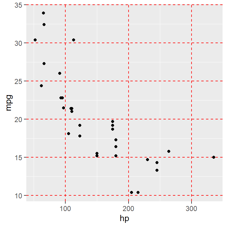
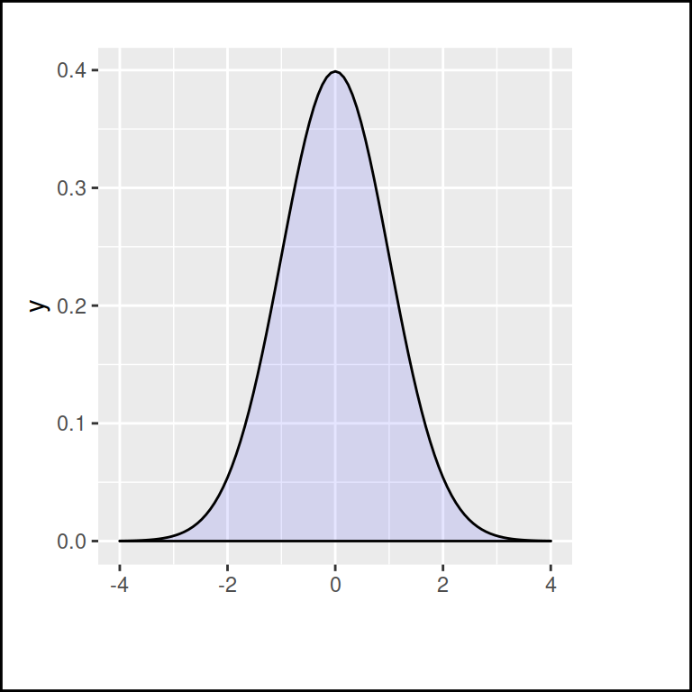
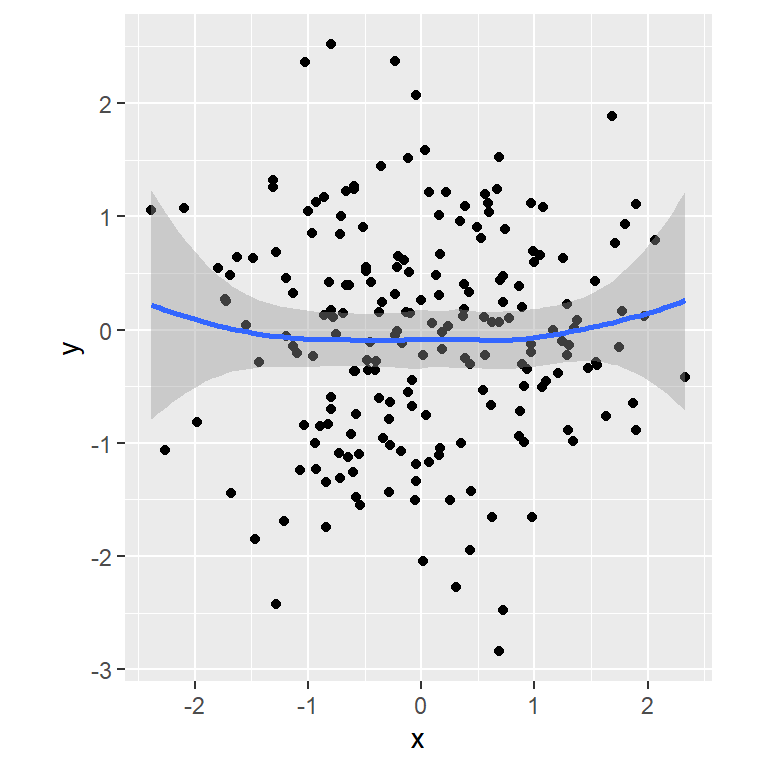
By default, ggplot2 charts have cartesian coordinate. However, the coord_cartesian function is very useful for zooming the plots, because if you use scale_x_continuous or scale_y_continuous the data will change the underlying data and hence the calculated stats, as shown below.
Default cartesian coordinates
# install.packages("ggplot2")
library(ggplot2)

# Data
set.seed(4)
df <- data.frame(x = rnorm(200),
                 y = rnorm(200))

p <- ggplot(df, aes(x = x, y = y)) +
  geom_point() +
  geom_smooth()

p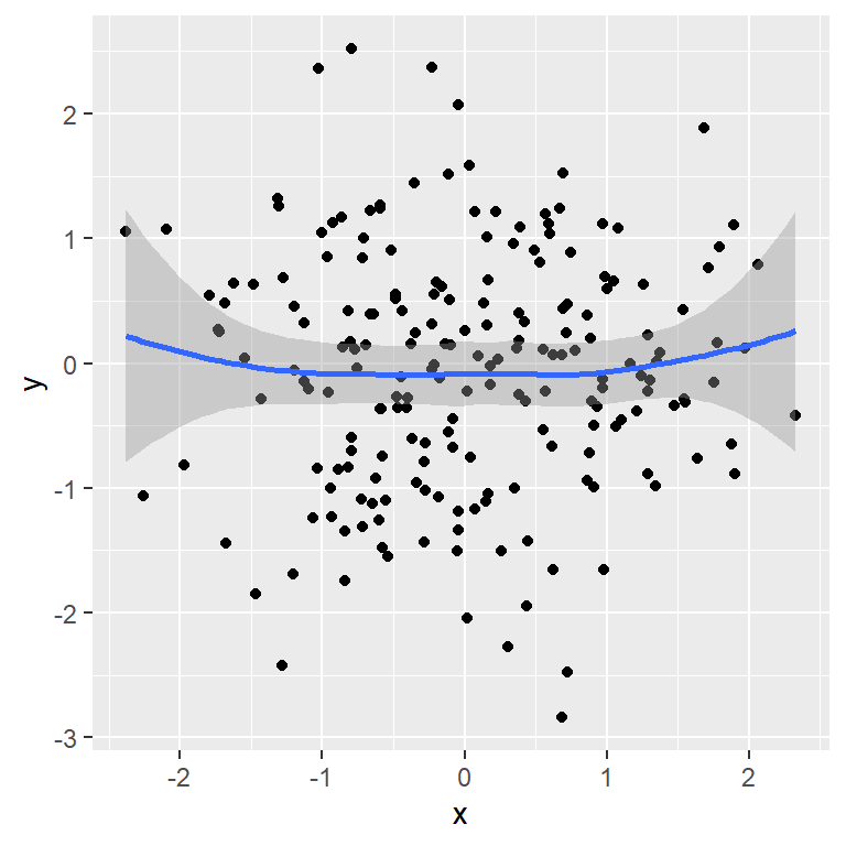
Using scale_x_continuous for zooming modifies the underlying data and the smooth estimation.
# install.packages("ggplot2")
library(ggplot2)

# Data
set.seed(4)
df <- data.frame(x = rnorm(200),
                 y = rnorm(200))

p <- ggplot(df, aes(x = x, y = y)) +
  geom_point() +
  geom_smooth()

p + scale_x_continuous(limits = c(-1, 1))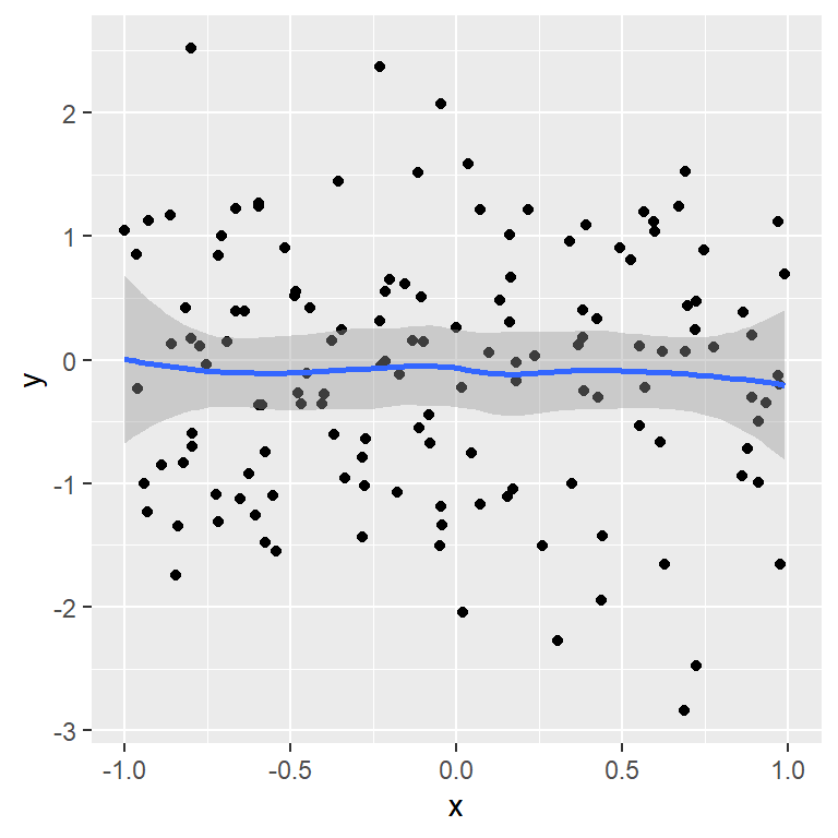
However, if you use coord_cartesian you can set the xlim and ylim without modifying the original estimations and just zooming in or out.
# install.packages("ggplot2")
library(ggplot2)

# Data
set.seed(4)
df <- data.frame(x = rnorm(200),
                 y = rnorm(200))

p <- ggplot(df, aes(x = x, y = y)) +
  geom_point() +
  geom_smooth()

p + coord_cartesian(xlim = c(-1, 1))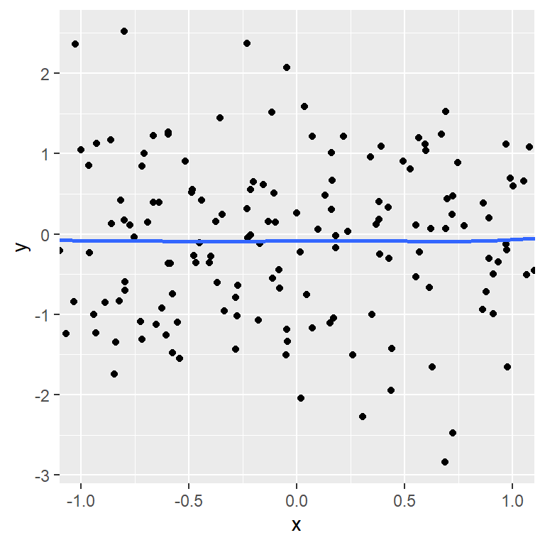
Fixed coordinates with coord_fixed
The coord_fixed function is very useful in case you want a fixed aspect ratio for your plot regardless the size of the plotting device. By default, one unit along the X axis will be the same unit along the Y axis, so the scales of the axes will be equal. You can use the ratio argument to specify the desired aspect ratio expressed as y/x.
# install.packages("ggplot2")
library(ggplot2)

# Data
set.seed(4)
df <- data.frame(x = rnorm(200),
                 y = rnorm(200))

p <- ggplot(df, aes(x = x, y = y)) +
  geom_point() +
  geom_smooth()

p + coord_fixed()
Flipping the axes with coord_flip
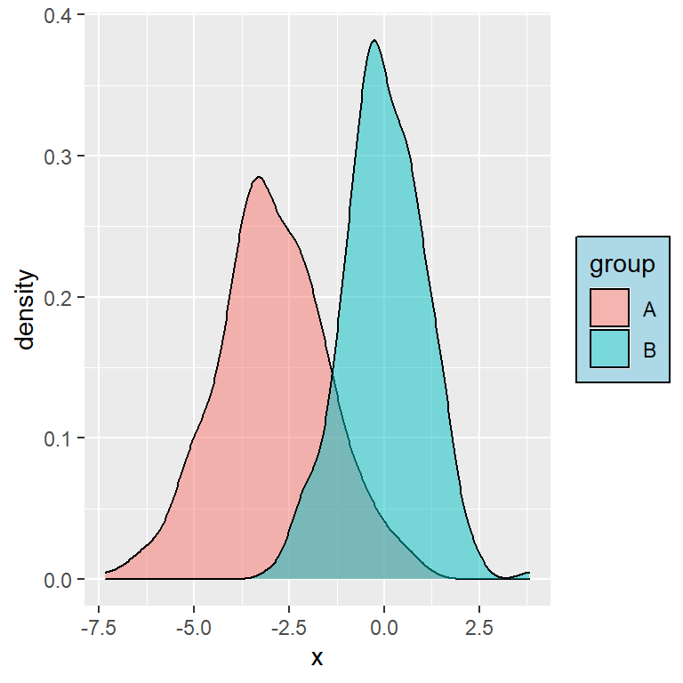
The coord_flip function rotates the axes in ggplot2, so if you have a vertical plot you can create the horizontal version and viceversa. This is specially useful for box plots, violin plots, …
Default
# install.packages("ggplot2")
library(ggplot2)

# Data
set.seed(4)
df <- data.frame(x = rnorm(200))

p <- ggplot(df, aes(x = x, y = "")) +
  geom_boxplot()

p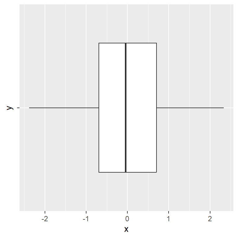
Flipped axes
# install.packages("ggplot2")
library(ggplot2)

# Data
set.seed(4)
df <- data.frame(x = rnorm(200))

p <- ggplot(df, aes(x = x, y = "")) +
  geom_boxplot()

p + coord_flip()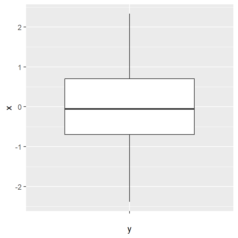
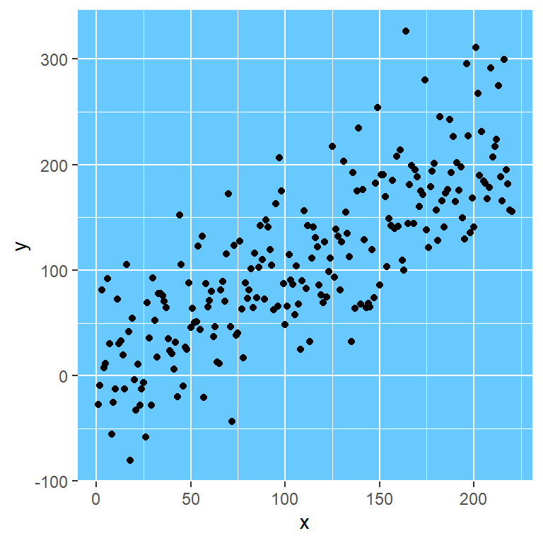
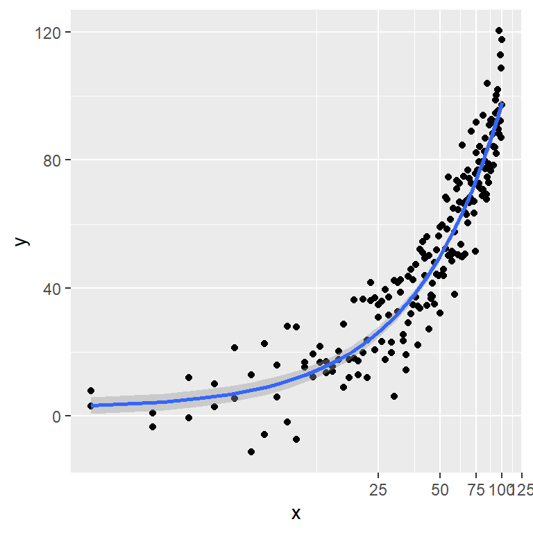
Transformations with coord_trans
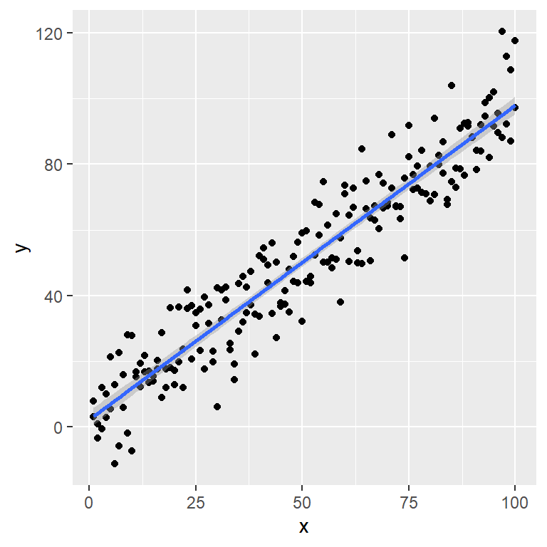
The coord_trans function creates transformed cartesian coordinate systems. Note that using this functions is not the same as transforming the scale, due to when using coord_trans the transformation occurs after statistics, affecting the visual appearance of geoms. Consider the following sample plot:
# install.packages("ggplot2")
library(ggplot2)

# Data
set.seed(4)
df <- data.frame(x = 1:100,
                 y = 1:100 + rnorm(200, sd = 10))

p <- ggplot(df, aes(x = x, y = y)) +
  geom_point() +
  geom_smooth(method = "lm")

p
In the following example we are transforming the X-axis (x argument) with the log function, so the linear estimate will become a curve. Recall that you can pass any function to the axes as long as it makes sense.
# install.packages("ggplot2")
library(ggplot2)

# Data
set.seed(4)
df <- data.frame(x = 1:100,
                 y = 1:100 + rnorm(200, sd = 10))

p <- ggplot(df, aes(x = x, y = y)) +
  geom_point() +
  geom_smooth(method = "lm")

p + coord_trans(x = "log")
Polar coordinates with coord_polar
The polar coordinates can be created using coord_polar. This type of coordinates are commonly used for pie charts (which are stacked bar charts in polar coordinates), wind roses, radar charts, bullseye charts, …
Note that by default the angle is mapped to the x variable, but you can set theta = "y" to map the angle to the y variable. You can also modify the direction of the plot with the direction argument (set -1 for anticlockwise). See the examples below for clarification.
# install.packages("ggplot2")
library(ggplot2)

# Data
set.seed(4)
df <- data.frame(x = 1:10,
                 y = sample(1:10))

p <- ggplot(df, aes(x = x, y = y, fill = y)) +
  geom_bar(stat = "identity", color = "white",
           lwd = 1, show.legend = FALSE)

p + coord_polar()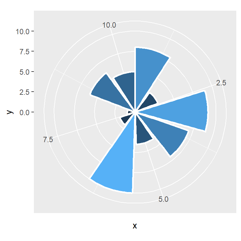
# install.packages("ggplot2")
library(ggplot2)

# Data
set.seed(4)
df <- data.frame(x = 1:10,
                 y = sample(1:10))

p <- ggplot(df, aes(x = x, y = y, fill = y)) +
  geom_bar(stat = "identity", color = "white",
           lwd = 1, show.legend = FALSE)

p + coord_polar(theta = "y")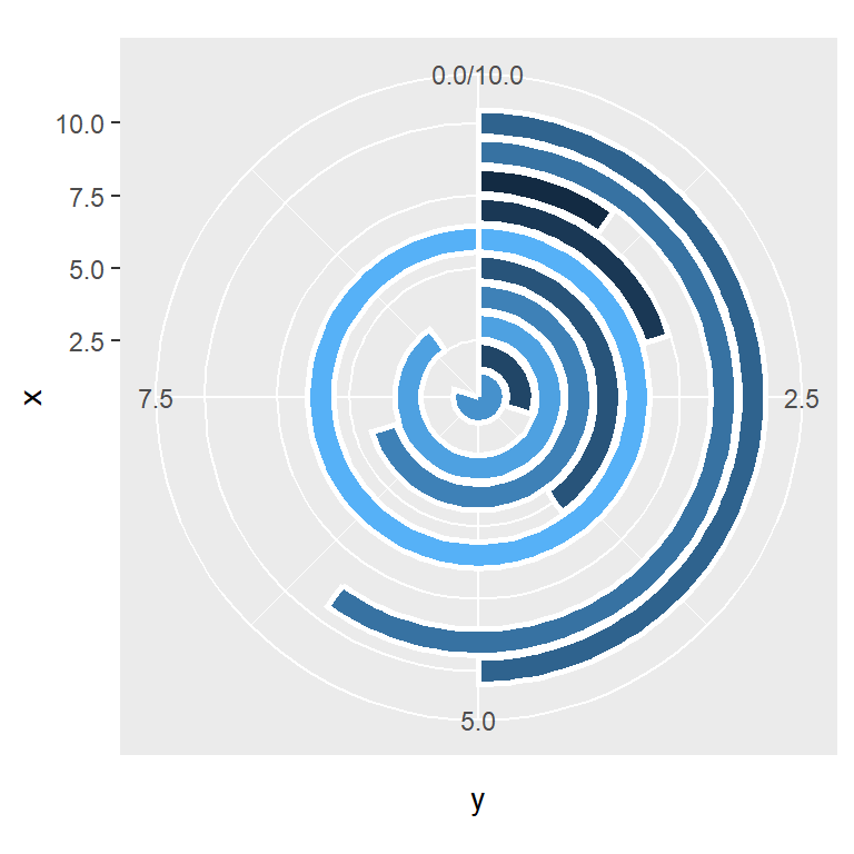
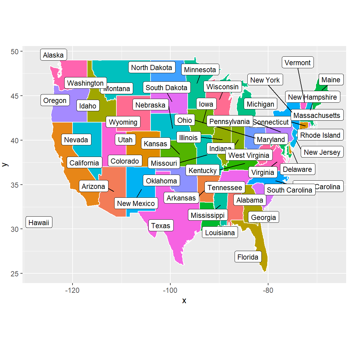
Map projections with coord_quickmap and coord_map
The last system coordinates are related to map projections. You will need to have the mapproj package installed in your computer for applying the projections.
On the one hand, the coord_map function requires considerable computation, but will approximate the projection as much as possible. Note that there are lots of different projections available. Type ?mapproj::mapproject for the full list.
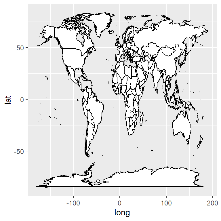
Default map
# install.packages("ggplot2")
library(ggplot2)
# install.packages("mapproj")

p <- ggplot(map_data("world"),
            aes(long, lat, group = group)) +
      geom_polygon(fill = "white", colour = 1)

p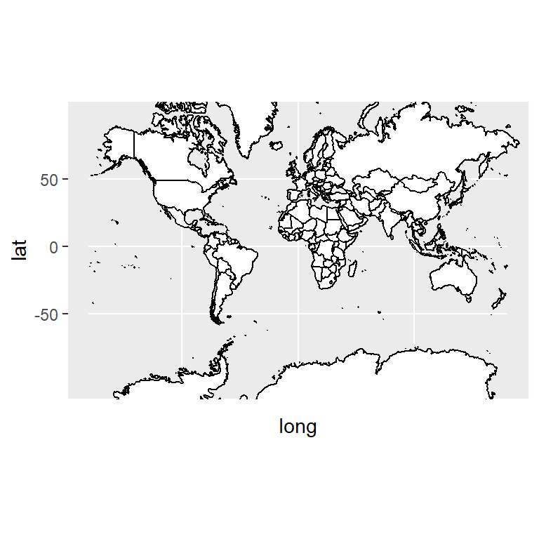
Mercator projection
The default projection is the well-known Mercator projection. Note that we modified the limits of the X-axis due to the function produces some unwanted horizontal lines. If you want to create this plot using coord_sf from sf package is a better solution.
# install.packages("ggplot2")
library(ggplot2)
# install.packages("mapproj")

p <- ggplot(map_data("world"),
            aes(long, lat, group = group)) +
      geom_polygon(fill = "white", colour = 1)

p + coord_map(xlim = c(-180, 180))
# p + sf::coord_sf() # Better solution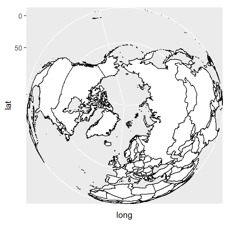
Orthographic projection
# install.packages("ggplot2")
library(ggplot2)
# install.packages("mapproj")

p <- ggplot(map_data("world"),
            aes(long, lat, group = group)) +
      geom_polygon(fill = "white", colour = 1)

p + coord_map("orthographic")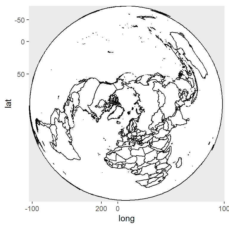
Fish eye
# install.packages("ggplot2")
library(ggplot2)
# install.packages("mapproj")

p <- ggplot(map_data("world"),
            aes(long, lat, group = group)) +
      geom_polygon(fill = "white", colour = 1)

p + coord_map("fisheye",
              n = 4) # Refractive index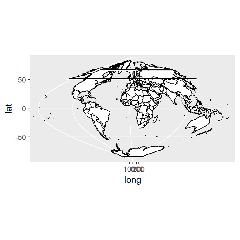
Sinusoidal
# install.packages("ggplot2")
library(ggplot2)
# install.packages("mapproj")

p <- ggplot(map_data("world"),
            aes(long, lat, group = group)) +
      geom_polygon(fill = "white", colour = 1)

p + coord_map("sinusoidal")
On the other hand, coord_quickmap also fixes the projection of a map, as shown below, but this function is a quick approximation for preserving straight lines which works best for small areas closer to the equator. Note that you can also apply any desired projection with the projection argument of the function, as in the previous examples.
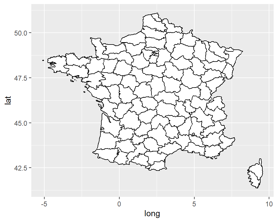
Default map
# install.packages("ggplot2")
library(ggplot2)

p <- ggplot(map_data("france"),
            aes(long, lat, group = group)) +
      geom_polygon(fill = "white", colour = 1)

p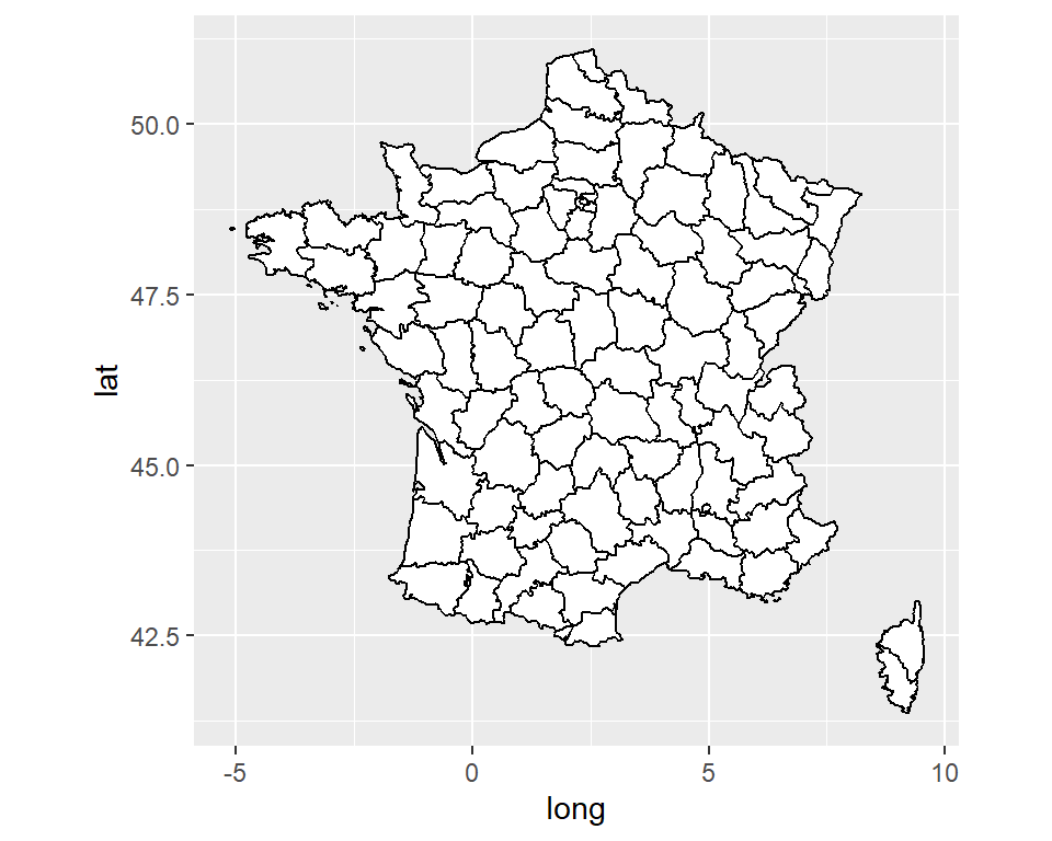
Fixing the projection
# install.packages("ggplot2")
library(ggplot2)

p <- ggplot(map_data("france"),
            aes(long, lat, group = group)) +
      geom_polygon(fill = "white", colour = 1)

p + coord_quickmap()
Master Statistics
Learn statistics from the basics to advanced techniques, clearly explained
Go to site