Interactive Sankey diagram in R with plotly

Package

Sample data

A Sankey diagram displays flows between nodes, where the width of each link is proportional to the size of the flow. In this tutorial we are going to use a data frame with the visits of a website, going from the source of the traffic to the pages of the site and from the pages to the final outcome.

plotly requires the nodes and the indices of the source and the target of each link. Create a data frame with the names of the nodes and use match to get the position of each source and target. Note that you need to subtract one, as plotly indices start at zero.

links <- data.frame(
  source = c("Organic search", "Organic search", "Social media", "Social media",
             "Email", "Email", "Blog", "Blog", "Product page", "Product page"),
  target = c("Blog", "Product page", "Blog", "Product page",
             "Blog", "Product page", "Product page", "Exit", "Purchase", "Exit"),
  value  = c(500, 300, 250, 100, 80, 170, 350, 480, 320, 600)
)

nodes <- data.frame(name = unique(c(links$source, links$target)))

links$source_id <- match(links$source, nodes$name) - 1
links$target_id <- match(links$target, nodes$name) - 1

Sankey diagram with plotly

Set type = "sankey" inside plot_ly and pass the labels of the nodes to node and the indices and the values of the links to link, both as lists. You can drag the nodes to rearrange them and hover over the links to see the size of each flow.

# install.packages("plotly")
library(plotly)

plot_ly(type = "sankey",
        node = list(label = nodes$name),
        link = list(source = links$source_id,
                    target = links$target_id,
                    value  = links$value))

Color of the nodes

The colors of the nodes are set with the color element of the node list. Pass a vector with as many colors as nodes, in the same order as in the data frame of the nodes.

cols <- c("#1B998B", "#ED217C", "#F4A259", "#2D3047", "#5B8E7D", "#BC4B51", "#3BB273")

plot_ly(type = "sankey",
        node = list(label = nodes$name,
                    color = cols),
        link = list(source = links$source_id,
                    target = links$target_id,
                    value  = links$value))

Color of the links

By default, the links are gray. A common approach is to color each link with the color of its source node adding some transparency. You can do it selecting the colors with the indices of the sources (adding one, as R indices start at one), getting their RGB values with col2rgb and creating rgba colors, where the last value is the transparency.

rgb_cols <- col2rgb(cols[links$source_id + 1])
link_cols <- sprintf("rgba(%d, %d, %d, 0.4)",
                     rgb_cols[1, ], rgb_cols[2, ], rgb_cols[3, ])

plot_ly(type = "sankey",
        node = list(label = nodes$name,
                    color = cols),
        link = list(source = links$source_id,
                    target = links$target_id,
                    value  = links$value,
                    color  = link_cols))

Size and border of the nodes

The node list also allows customizing the separation between the nodes with pad, their width with thickness and their border with line, which takes a list with the color and the width of the border.

plot_ly(type = "sankey",
        node = list(label = nodes$name,
                    color = cols,
                    pad = 30,
                    thickness = 12,
                    line = list(color = "white", width = 2)),
        link = list(source = links$source_id,
                    target = links$target_id,
                    value  = links$value,
                    color  = link_cols))

Hover text

The text displayed when hovering over the links can be customized with hovertemplate, using %{source.label}, %{target.label} and %{value}. In addition, you can add a suffix to the values with valuesuffix and change the title and the font with layout.

plot_ly(type = "sankey",
        valuesuffix = " visits",
        node = list(label = nodes$name,
                    color = cols),
        link = list(source = links$source_id,
                    target = links$target_id,
                    value  = links$value,
                    color  = link_cols,
                    hovertemplate = "%{source.label} to %{target.label}<br>%{value}<extra></extra>")) |>
  layout(title = "Website traffic", font = list(size = 12))

Vertical Sankey diagram

Set orientation = "v" to create a vertical Sankey diagram, where the flows go from top to bottom. This orientation is useful when there are many stages or when the names of the nodes are long.

plot_ly(type = "sankey",
        orientation = "v",
        node = list(label = nodes$name,
                    color = cols),
        link = list(source = links$source_id,
                    target = links$target_id,
                    value  = links$value,
                    color  = link_cols))

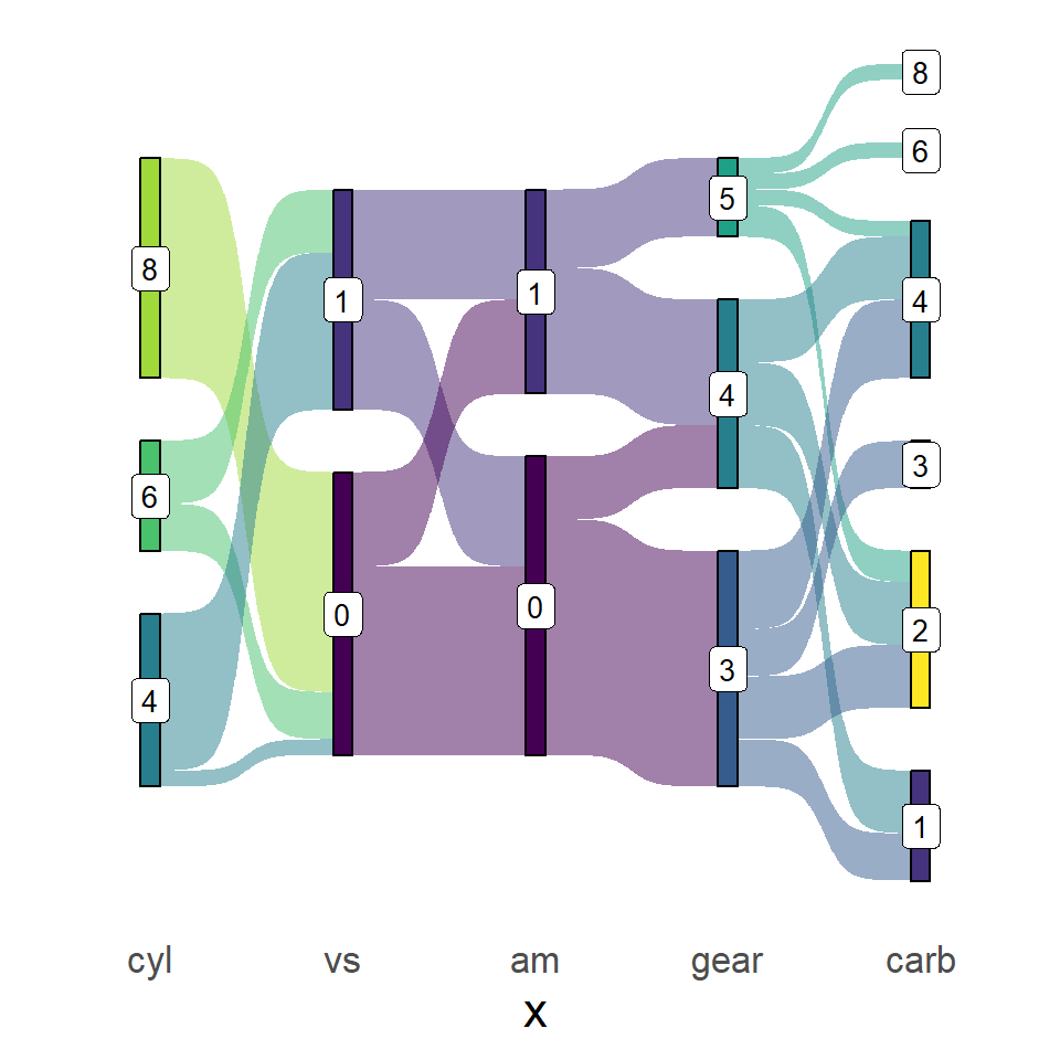
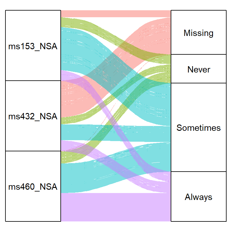
If you prefer static charts you can create a Sankey diagram in ggplot2 or an alluvial plot. Check the guide about interactive plots with plotly to learn more about the package.