The plot_usmap function
The usmap package allows creating maps of the United States in R in a very simple way. Its main advantage is that Alaska and Hawaii are placed under the rest of the states, so the map is compact, and that the maps are ggplot2 objects, so you can customize them with the usual ggplot2 functions.
Use the plot_usmap function to plot the map. By default, the function displays the states, but you can display the counties setting regions = "counties".
# install.packages("usmap")
library(usmap)

plot_usmap()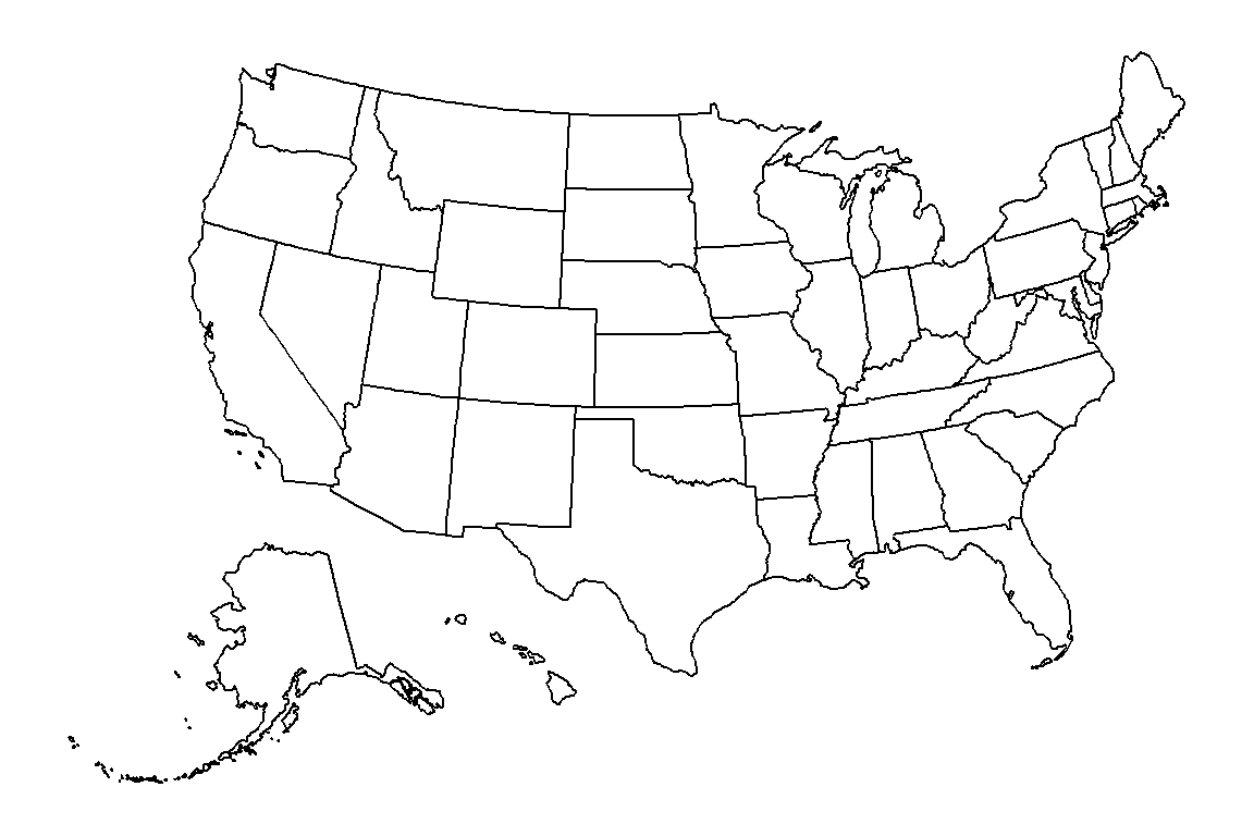
Counties
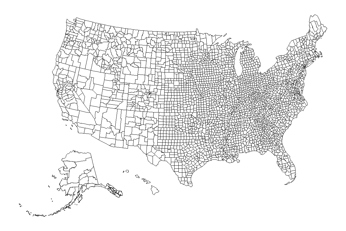
Set regions = "counties" to plot the borders of the counties. As there are more than 3000 counties you may want to reduce the width of the borders with linewidth.
plot_usmap(regions = "counties", linewidth = 0.1)Select states or regions
The include and exclude arguments allow selecting the states to display, passing their abbreviations, names or FIPS codes. The package also provides vectors with the states of each region, such as .west_region, .south_region, .northeast_region or .midwest_region.
plot_usmap(include = .west_region,
           fill = "#E8D5B7", color = "#6B2737")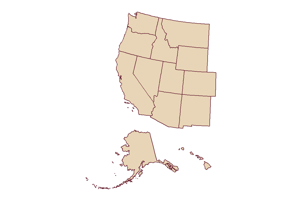
Counties of a state
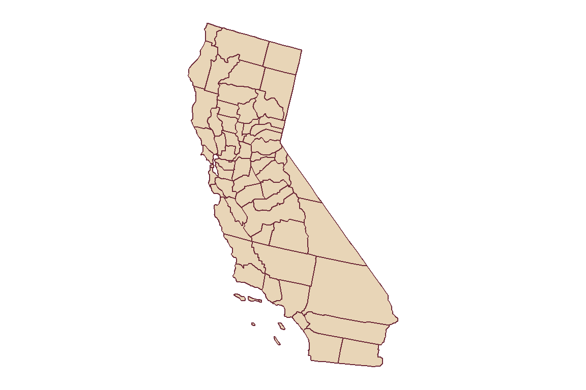
You can combine both arguments to display the counties of one or several states. In this example we are plotting the counties of California.
plot_usmap(regions = "counties", include = "CA",
           fill = "#E8D5B7", color = "#6B2737")
Choropleth map
In order to create a choropleth map you will need a data frame with a column named fips or state (or county for county maps) and a column with the values. Pass the data frame to data and the name of the column to values. In this example we are using the statepop data set, which contains the population of each state.
plot_usmap(data = statepop, values = "pop_2022", color = "white") +
  scale_fill_gradient(low = "#FFE8D6", high = "#6B2737",
                      name = "Population", label = scales::comma) +
  theme(legend.position = "right")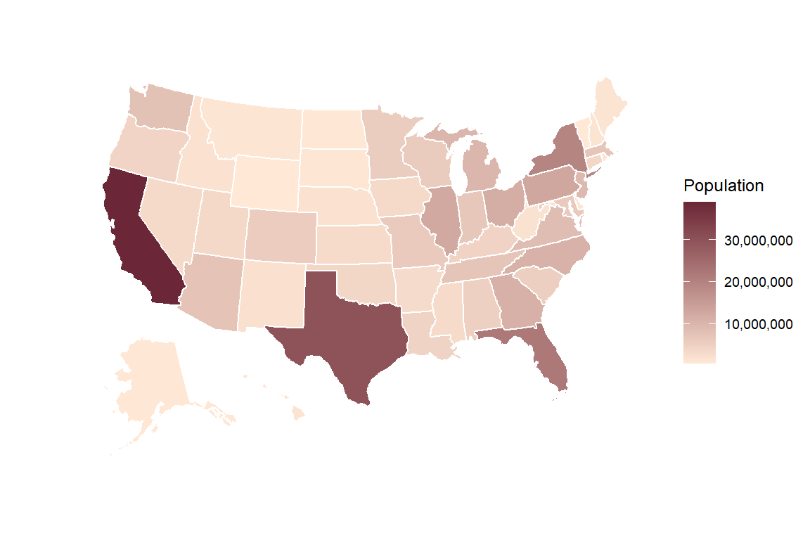
As the output is a ggplot2 object, the colors of the map are set with the usual scales, such as scale_fill_gradient or scale_fill_viridis_c, and the legend is customized with the theme function.
Choropleth map by county
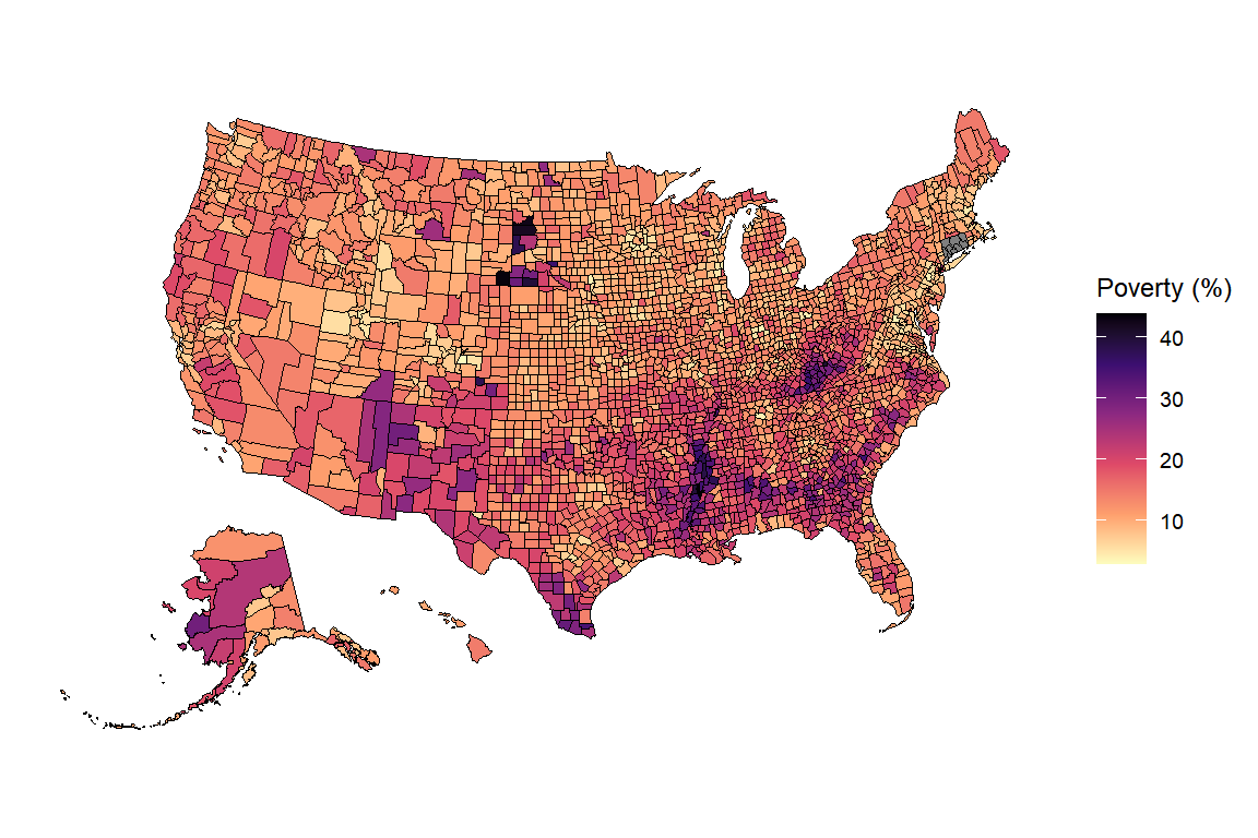
The same can be done with the counties. The countypov data set contains the percentage of people in poverty of each county in 2021, identified by its FIPS code.
plot_usmap(regions = "counties", data = countypov, values = "pct_pov_2021",
           linewidth = 0.05) +
  scale_fill_viridis_c(name = "Poverty (%)", option = "magma", direction = -1) +
  theme(legend.position = "right")
Labels
Set labels = TRUE to display the abbreviations of the states (or the names of the counties) and use label_color to change their color. Note that the labels of the small states of the northeast will overlap.
plot_usmap(data = statepop, values = "pop_2022", color = "white",
           labels = TRUE, label_color = "white") +
  scale_fill_gradient(low = "#E8A87C", high = "#6B2737") +
  theme(legend.position = "none")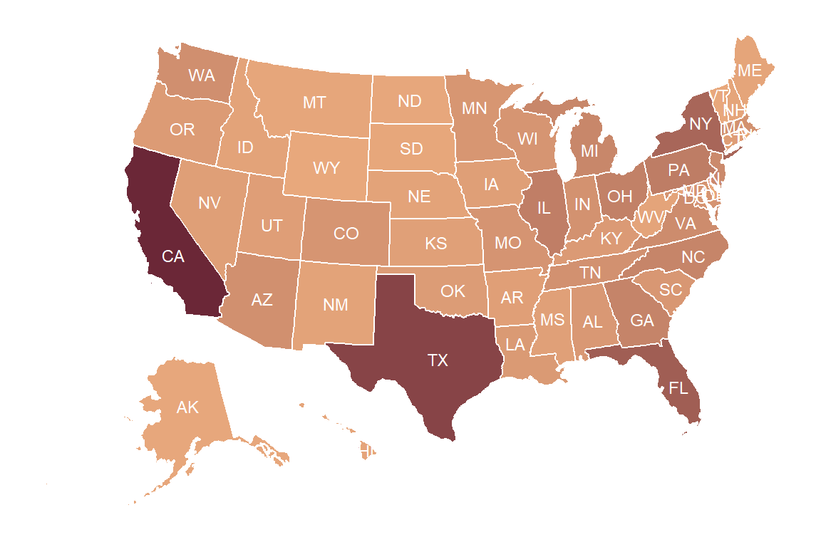
Add points to the map
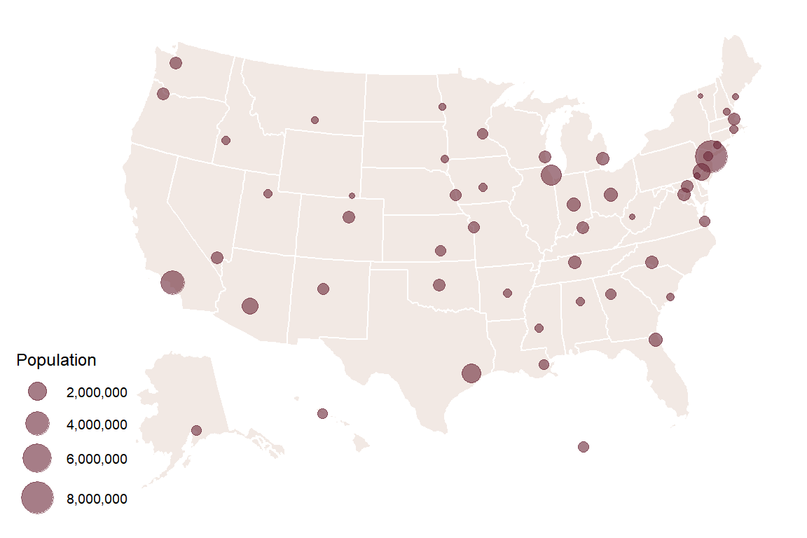
If you want to add points to the map you will need to transform the coordinates (longitude and latitude) to the projection used by usmap with usmap_transform. Then, add them with geom_sf. In this example we are using the citypop data set, which contains the coordinates and the population of the most populous city of each state.
cities <- usmap_transform(citypop)

plot_usmap(fill = "#F2E9E4", color = "white") +
  geom_sf(data = cities, aes(size = city_pop),
          color = "#6B2737", alpha = 0.6) +
  scale_size_continuous(range = c(1, 8), label = scales::comma,
                        name = "Population")
If you want to create maps of other countries check how to create maps in ggplot2 and choropleth maps in ggplot2. For interactive maps you can use leaflet.
Master Statistics
Learn statistics from the basics to advanced techniques, clearly explained
Go to site