Sample data
The corrplot package allows visualizing correlation matrices in R in a very simple way. It provides several visualization methods and options to reorder the variables, show only half of the matrix, display the correlation coefficients or highlight the significant correlations.
In this tutorial we are going to use the correlation matrix of the variables of the mtcars data set, computed with the cor function. Note that corrplot requires a correlation matrix, not the raw data, so you will need to compute it first.
M <- cor(mtcars)
The corrplot function
Pass the correlation matrix to the corrplot function to create a correlation plot. By default, each correlation is represented with a circle whose size and color depend on the value of the correlation: blue for positive correlations and red for negative correlations.
# install.packages("corrplot")
library(corrplot)

corrplot(M)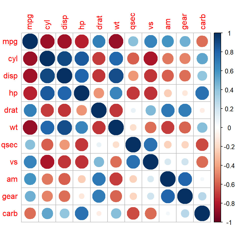
Visualization method
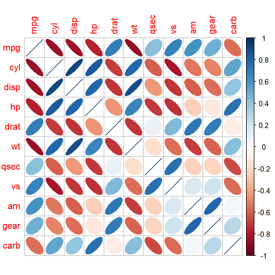
The method argument allows choosing how to represent the correlations. The available options are "circle" (default), "square", "ellipse", "number", "shade", "color" and "pie". In the following example we are using ellipses, which are narrower the stronger the correlation is.
corrplot(M, method = "ellipse")If you prefer a heat map you can set method = "color", which fills each cell with the color corresponding to the correlation. This method is very useful when combined with the correlation coefficients, as shown in the following sections.
corrplot(M, method = "color")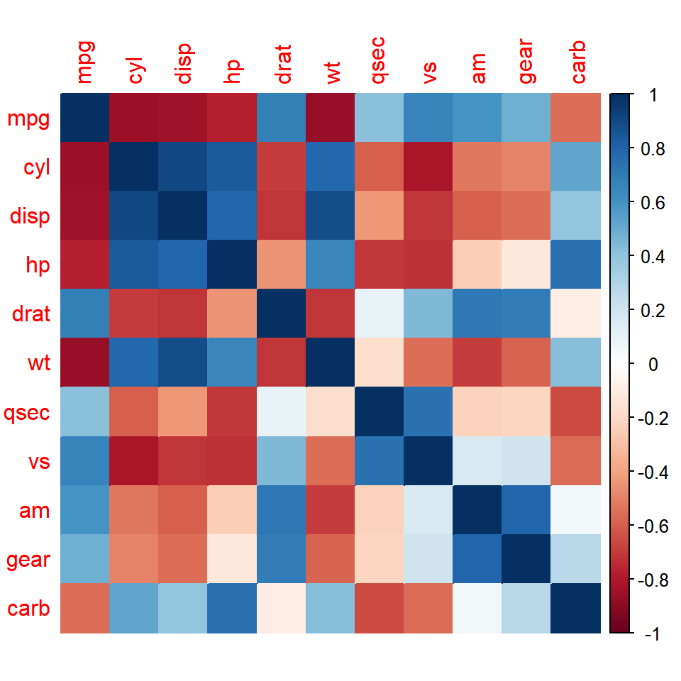
Upper or lower triangle
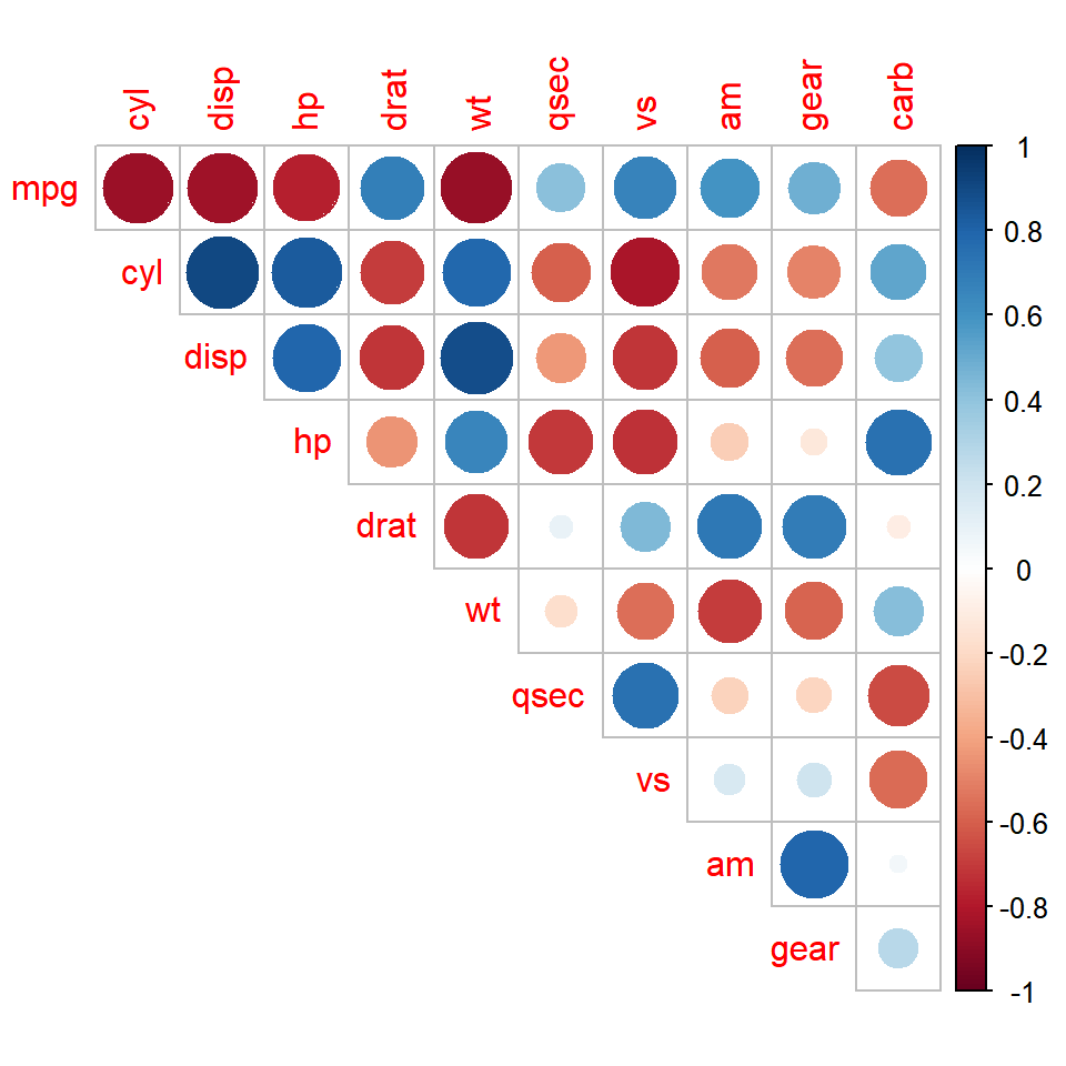
As the correlation matrix is symmetric, you can display only one half of it with type = "upper" or type = "lower". In addition, the diagonal only contains ones (the correlation of each variable with itself), so you can remove it with diag = FALSE.
corrplot(M, type = "upper", diag = FALSE)Reorder the variables
By default, the variables are displayed in the same order as in the matrix. The order argument allows reordering them to make the patterns easier to see. The options are "original", "AOE" (angular order of the eigenvectors), "FPC" (first principal component), "hclust" (hierarchical clustering) and "alphabet".
When using order = "hclust" you can also draw rectangles around the clusters with addrect, specifying the number of clusters. The clustering method can be changed with hclust.method.
corrplot(M, order = "hclust", addrect = 2)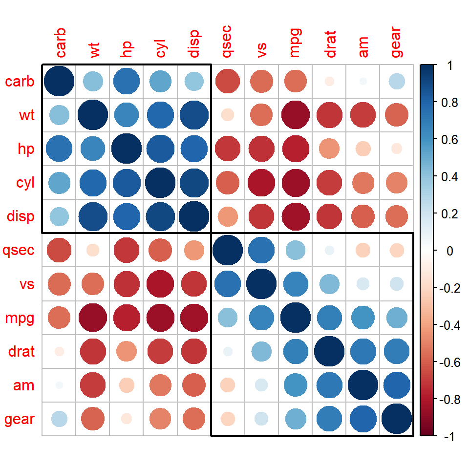
Correlation coefficients
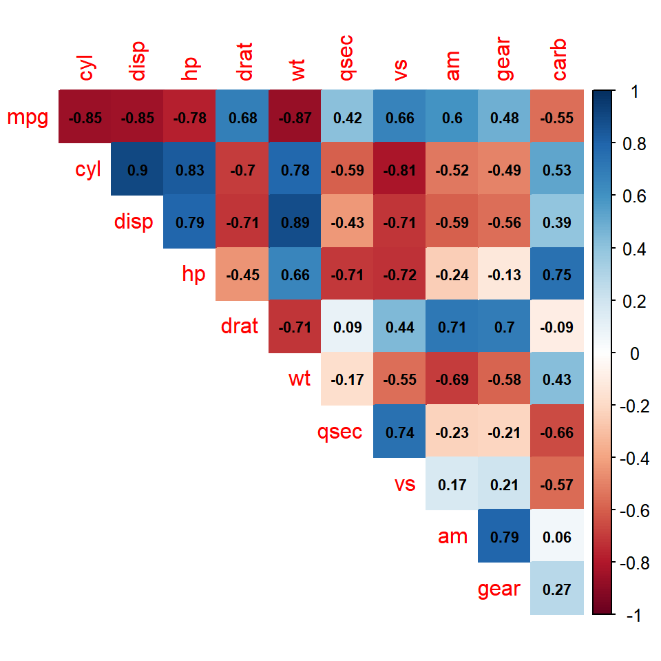
The correlation coefficients can be added over the plot with addCoef.col, which sets the color of the numbers, while their size can be changed with number.cex. If you only want to display the numbers use method = "number" instead.
corrplot(M, method = "color", type = "upper", diag = FALSE,
         addCoef.col = "black", number.cex = 0.7)
Mixed correlation plot
The corrplot.mixed function allows using a different method for each half of the matrix. By default, the lower triangle displays the correlation coefficients and the upper triangle displays circles, but you can change them with the lower and upper arguments.
corrplot.mixed(M, lower = "number", upper = "ellipse",
               tl.col = "black", number.cex = 0.7)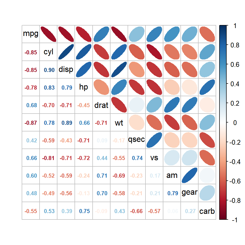
Significance of the correlations
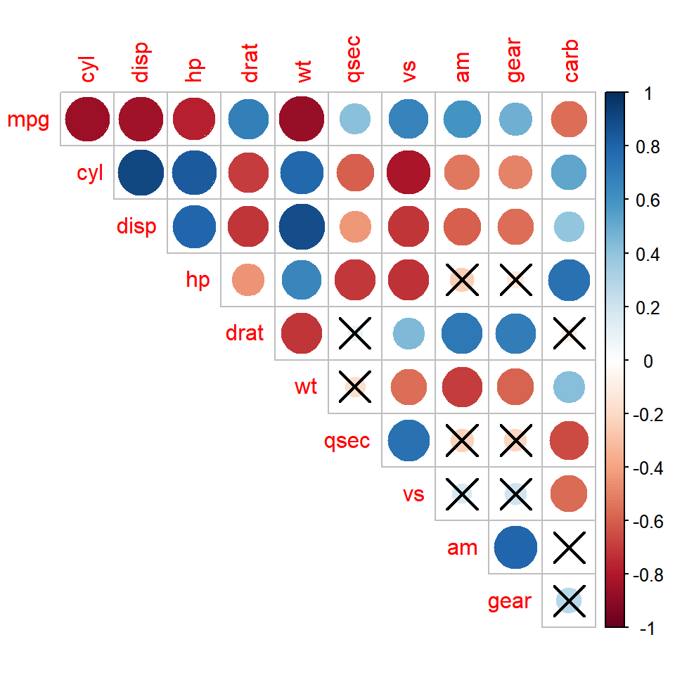
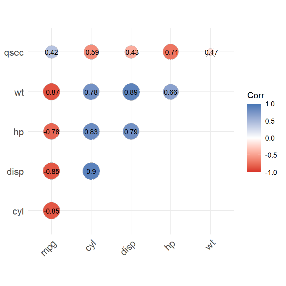
The cor.mtest function computes the p-values of the correlation tests for each pair of variables. Pass the matrix of p-values to p.mat and set the significance level with sig.level to cross out the non-significant correlations. If you prefer to remove them set insig = "blank".
p <- cor.mtest(mtcars, conf.level = 0.95)

corrplot(M, type = "upper", diag = FALSE,
         p.mat = p$p, sig.level = 0.05)
Colors
The color palette can be customized with the col argument. corrplot includes the COL1 (sequential) and COL2 (diverging) functions, which provide palettes from RColorBrewer, such as "RdBu", "PiYG" or "PuOr". You can also create your own palette with colorRampPalette or choose other color palettes.
corrplot(M, type = "upper", diag = FALSE,
         col = COL2("PuOr"))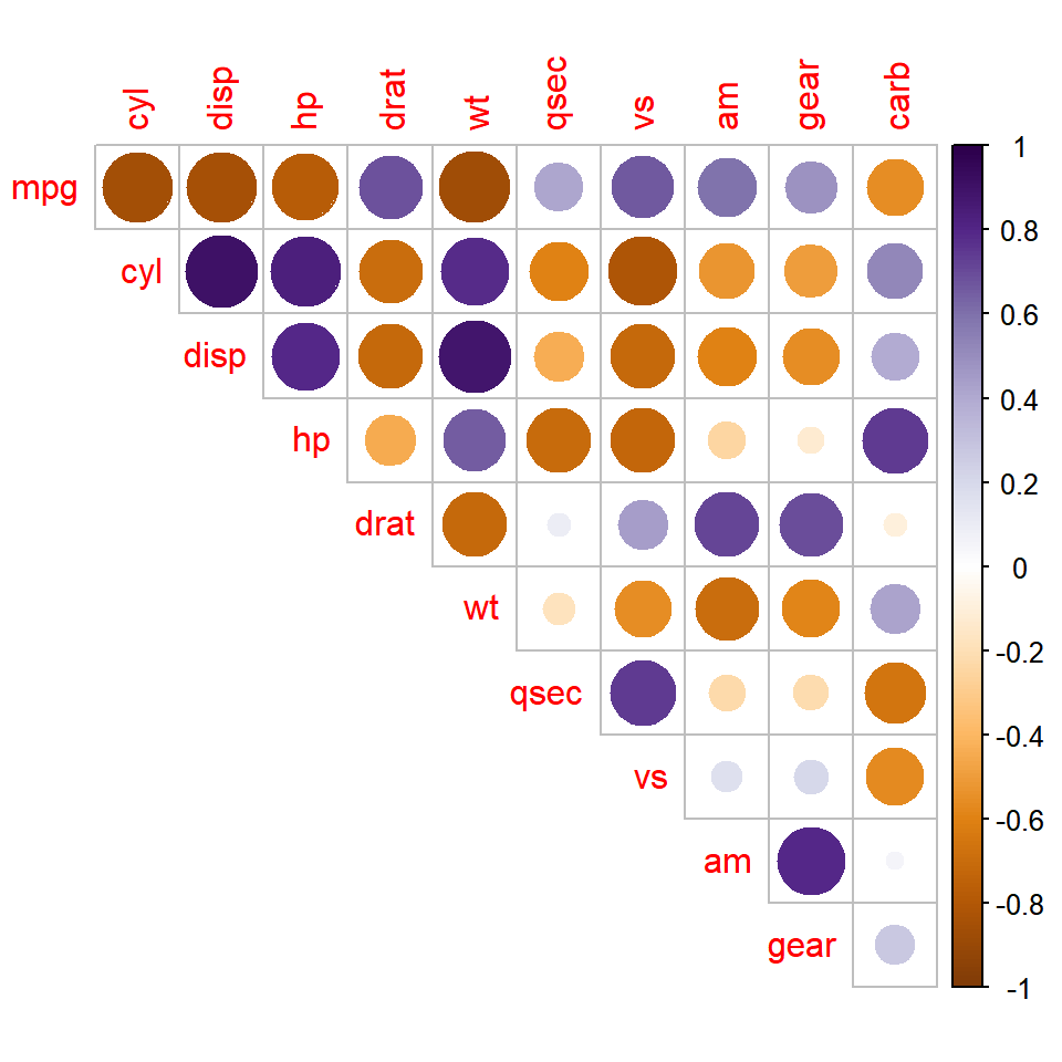
Labels and legend
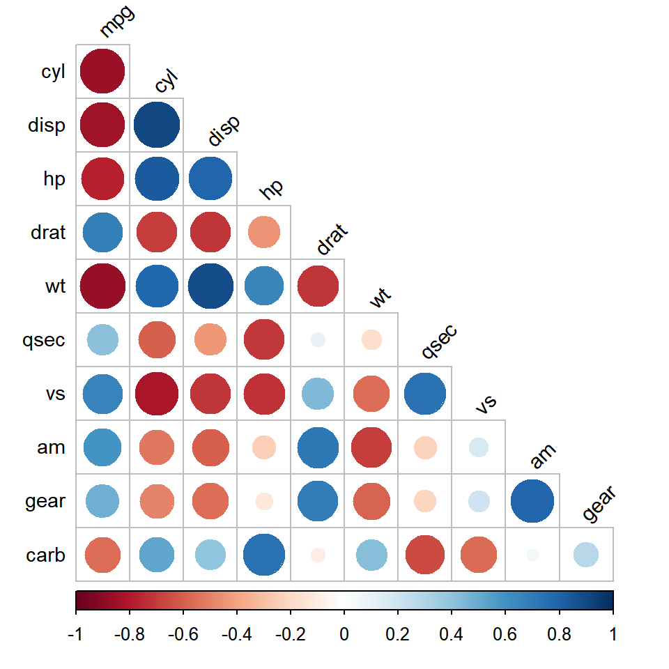
The arguments starting with tl allow customizing the text labels: tl.col sets the color, tl.srt the rotation and tl.cex the size. The position of the color legend can be changed with cl.pos, which can be "r" (right), "b" (bottom) or "n" (no legend).
corrplot(M, type = "lower", diag = FALSE,
         tl.col = "black", tl.srt = 45, tl.cex = 0.9,
         cl.pos = "b")
If you prefer ggplot2 you can create a correlation matrix with ggcorrplot or a heat map with geom_tile. In addition, if you want to display the scatter plots of each pair of variables along with the correlations check the ggpairs function. Note that the corrplot package is different from the corPlot function of the psych package.
Master Statistics
Learn statistics from the basics to advanced techniques, clearly explained
Go to site