Phylogenetic trees in R with ggtree

Package

Sample data

The ggtree package allows plotting and annotating phylogenetic trees using the grammar of ggplot2, so you can add layers to the tree as in any other ggplot2 chart. It is a Bioconductor package, so you will need the BiocManager package to install it.

In this tutorial we are going to use the bird.orders data set of the ape package, which contains the phylogenetic tree of the 23 orders of birds. If you have your own tree in a Newick file you can import it with the read.tree function of ape or with the treeio package, which supports other formats.

# install.packages("ape")
library(ape)

data(bird.orders)
tree <- bird.orders

# Your own tree:
# tree <- read.tree("tree.nwk")

## 
## Phylogenetic tree with 23 tips and 22 internal nodes.
## 
## Tip labels:
##   Struthioniformes, Tinamiformes, Craciformes, Galliformes, Anseriformes, Turniciformes, ...
## 
## Rooted; includes branch lengths.

The `ggtree` function

Pass the tree to the ggtree function to plot it and add the names of the tips with geom_tiplab. Note that the labels can be cut, so you may need to increase the limits of the X-axis with xlim.

# install.packages("BiocManager")
# BiocManager::install("ggtree")
library(ggtree)

ggtree(tree) +
  geom_tiplab(size = 3) +
  xlim(0, 40)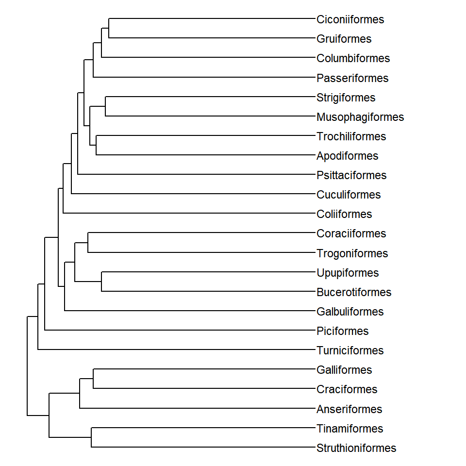

Phylogenetic tree in R with ggtree

Layout of the tree

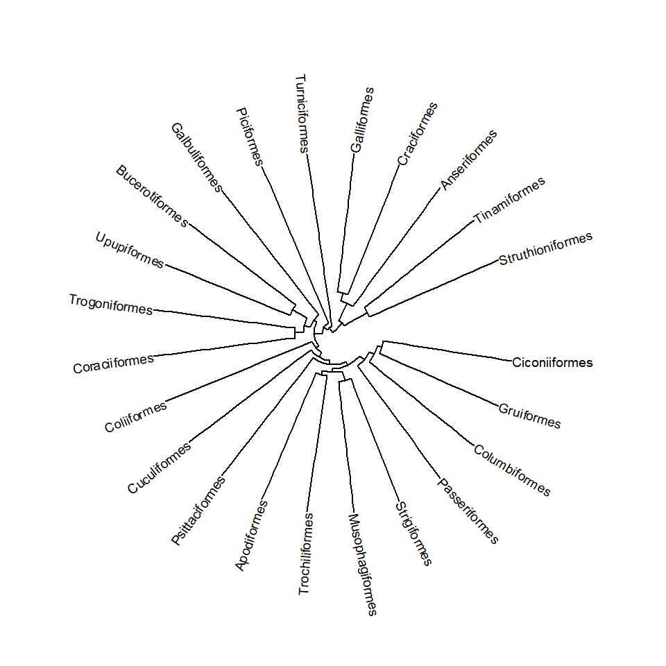
Circular phylogenetic tree with ggtree

The layout argument changes the shape of the tree. The default is "rectangular", but you can also use "slanted", "ellipse", "roundrect", "fan", "circular", "radial", "equal_angle" or "daylight". In this example we are creating a circular tree.

ggtree(tree, layout = "circular") +
  geom_tiplab(size = 2.5) +
  xlim(0, 40)

Tip and node points

The geom_tippoint and geom_nodepoint functions add points to the tips and to the internal nodes of the tree, respectively. As in ggplot2, you can customize their color, size and shape. The width of the branches can be changed with linewidth.

ggtree(tree, linewidth = 0.7) +
  geom_tippoint(color = "#33658A", size = 2.5) +
  geom_nodepoint(color = "#F26419", size = 2) +
  geom_tiplab(size = 3, offset = 0.5) +
  xlim(0, 40)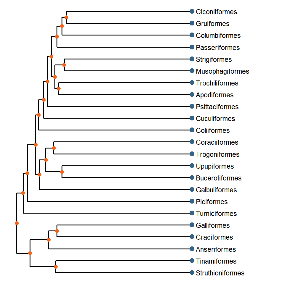

Phylogenetic tree with points in the tips and nodes with ggtree

Node numbers

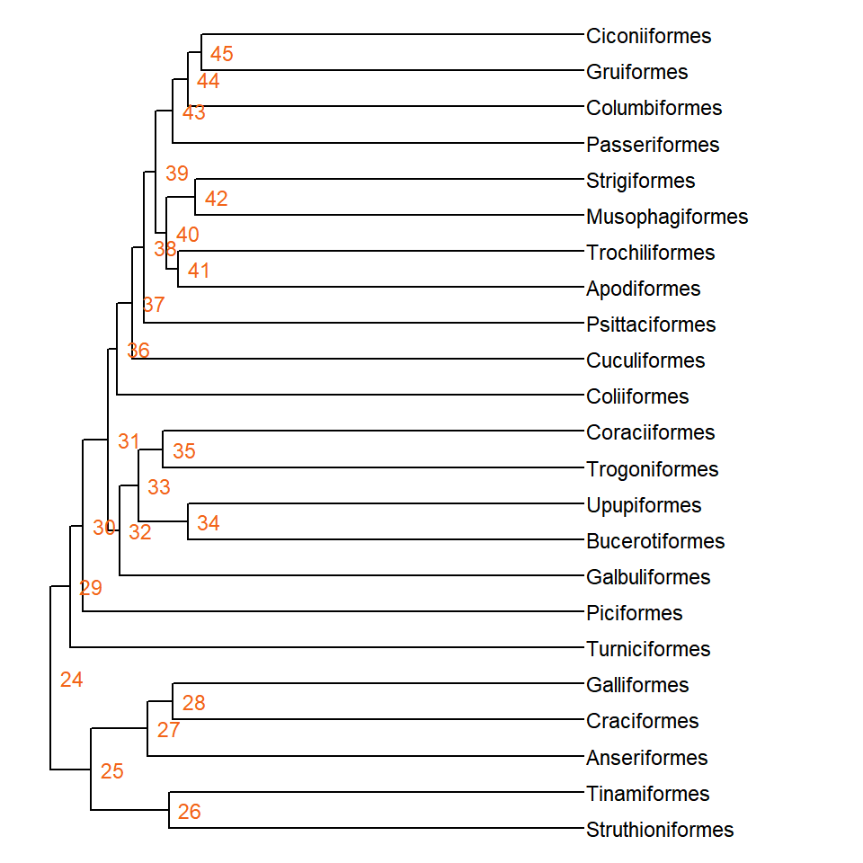
Phylogenetic tree with the numbers of the nodes in ggtree

In order to annotate a clade you will need the number of its node. You can display the numbers of the internal nodes with geom_nodelab(aes(label = node)) or get the node of the most recent common ancestor of several tips with the getMRCA function of ape, such as getMRCA(tree, c("Struthioniformes", "Tinamiformes")).

ggtree(tree) +
  geom_tiplab(size = 3) +
  geom_nodelab(aes(label = node), hjust = -0.3, size = 3, color = "#F26419") +
  xlim(0, 40)

Highlight clades

geom_hilight highlights a clade with a rectangle, passing the number of its node to node, and geom_cladelab adds a bar with a label to its right. In this example we are highlighting the three main groups of birds: Palaeognathae (ostriches and tinamous), Galloanserae (fowl and ducks) and Neoaves (the rest of the birds).

ggtree(tree) +
  geom_tiplab(size = 2.5) +
  geom_hilight(node = 26, fill = "#F6AE2D", alpha = 0.3) +
  geom_hilight(node = 27, fill = "#33658A", alpha = 0.3) +
  geom_hilight(node = 29, fill = "#F26419", alpha = 0.3) +
  geom_cladelab(node = 26, label = "Palaeognathae", offset = 9, fontsize = 3) +
  geom_cladelab(node = 27, label = "Galloanserae", offset = 9, fontsize = 3) +
  geom_cladelab(node = 29, label = "Neoaves", offset = 9, fontsize = 3) +
  xlim(0, 50)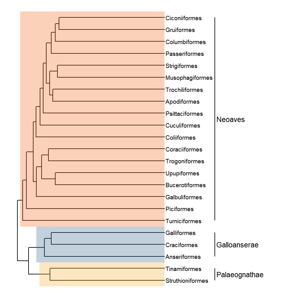

Highlight clades in a phylogenetic tree with ggtree

Color by clade

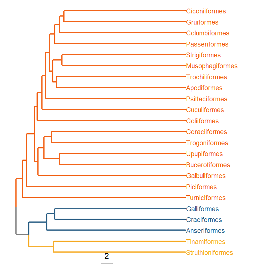
Color the branches of a phylogenetic tree by clade with ggtree

If you want to color the branches by clade use the groupClade function, which adds a group variable to the tree with the clade of each branch, and map it to color inside aes. The colors can be set with scale_color_manual, as in any other ggplot2 chart. Note that the first group (0) contains the branches that don’t belong to any clade. We are also adding a scale for the branch lengths with geom_treescale.

tree_groups <- groupClade(tree, .node = c(26, 27, 29))

ggtree(tree_groups, aes(color = group), linewidth = 0.8) +
  geom_tiplab(size = 3) +
  scale_color_manual(values = c("gray50", "#F6AE2D", "#33658A", "#F26419")) +
  geom_treescale() +
  xlim(0, 40) +
  theme(legend.position = "none")

If you need to plot the result of a hierarchical clustering instead of a phylogenetic tree check how to create a dendrogram with hclust or a circular dendrogram.